This is a friendly summary and critical review of the paper “Entropy-SGD: Biasing GD Into Wide Valleys” by Chaudhari et al. (2017) [1].
The post is designed to incrementally deepen the analysis and your understanding of the paper (i.e. you can read the first parts and you will have a birds eye view of what the paper is about).
However, by reading this post in its entirety you will, hopefully, understand the following:
- The core problem that motivated this paper.
- The historical background and research upon which this paper is based. I highly encourage you to read the papers that I cite. They formulate the foundation of understanding this paper and other methodologically similar papers.
- Summarize the important points of the methodology and the algorithm that is utilized.
- Important caveats that are not adequately stressed in the paper, especially with respect to the algorithm.
- Omissions that should have been included in the paper
- Assumptions, especially the one’s that are referenced.
- Theoretical properties of the paper and methods of proof.
- Resources for the mathematical notation, which is heavily influenced by statistical physics.
Introduction
The authors derive a different Stochastic Gradient Descent (henceforth SGD), which they label as “Entropy – SGD”. The change lies in a modification of the Loss Function of the optimization algorithm. Specifically, they render the the Loss Function “smoother”.
Motivation
Why do they make the Loss Function “smoother”? So that we have “flat minima” (or “wide valleys” as the authors write, the two terms can be used interchangeably).
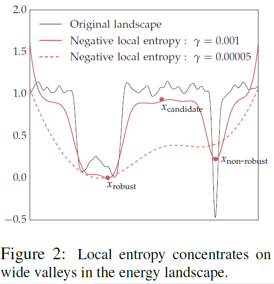
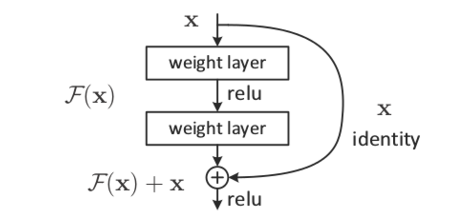
Let’s see what this cryptic notion of “flat minima” is all about. Watch carefully the following Figures 1 and 2.
Figure 1
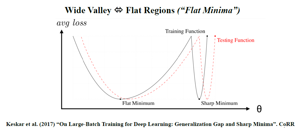
Figure 2
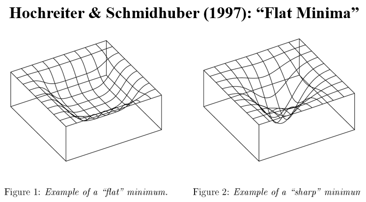
When we are in a region characterized as “flat minima”, the Loss Function changes more slowly. It is hypothesized that flat minima are “generalized” better. Thus, the motivation is to “bias” the objective function so that we end up with more “flat minima” (or “wide valleys”). This where the title of the paper partially comes from.
Now what do they mean by “generalized”? They refer to the “generalization error” (also known as the “out of sample error”). It is also refers on the concept “stability”, which I will discuss analytically.
Modify (Bias) the SGD
The modification (or biasing) of the SGD is by utilizing the concept of the local entropy. The were motivated by Baldassi et al. (2016) [2] who use “Local entropy as a measure for sampling solutions in constraint satisfaction problems”.
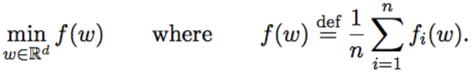
The goal is to maximize (or minimize its negative) the following Equation 1:
Equation 1
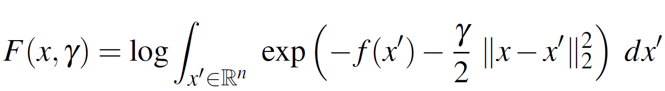
This components of Equation 1 are as follows:
 is the log partition function.
- The “depth” of the “valley” at a location

- The “flatness” is measured through the (local) entropy

- The hyper-parameter γ looks for “valleys” of specific “width”.
Intuition of Equation 1: “Bias” the optimization towards “wide (flat) valleys”.
The γ parameter
Let’s see the what γ does in practice. Figure 3 illustrates what happens to the loss function, the local entropy, when we increase γ. It becomes more “smooth”. Note that in Figure 3, the x-axis is the parameter space, the y-axis is the negative local entropy.
Figure 3
The Probabilistic Foundations
This is the point where we go deeper (learning sic).
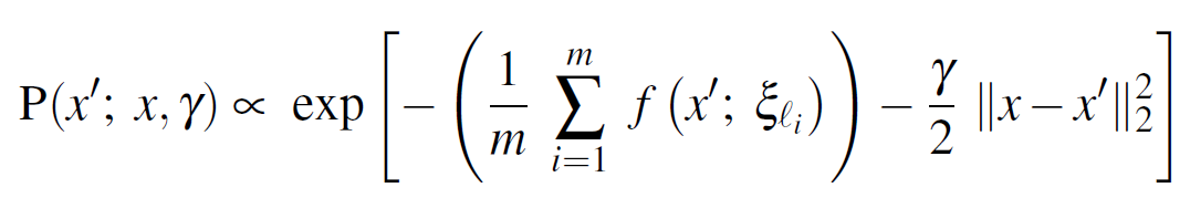
The probabilistic foundations of local entropy lie in Equation 2:
Equation 2
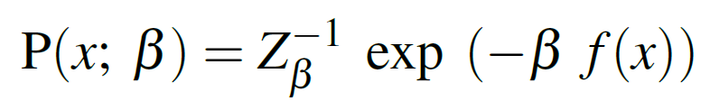
This is a conditional probability with the following properties:
- For an parameter vector
- Consider a Gibbs-Sampling Distribution where:
 : is the energy landscape
- β is the inverse “temperature” (see “Langevin dynamics”)
- Z is a regularization term.
The reason we have these cryptic terms (“temperature”?) is because this is a mathematical modeling that is used in in physics, specifically the mathematical modeling of molecular systems. Not so cryptic.
Intuition: When  , the probability distribution concentrates to the global minimum of
  .
.
However, this is the gist: the authors want “flat regions”. Subsequently, they need a Modified Gibbs-Sampling Distribution, specifically the Equation 2 is modified into Equation 3:
Equation 3
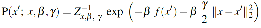
Equation 3 is a conditional probability with the following terms:
- γ which “biases” toward x .
- Large γ
 all the “mass” concentrates near
  regardless of
  energy term (which measures “flatness” as discussed
- Small γ
 dominates
- The authors set β=1, therefore β is a nuisance term.
- Instead, they focus on tuning γ
Revisiting the γ parameter: “scoping”
What Equation 3 tells us is that γ determines the “scope”. Specifically, in a neighborhood (region) around “x” (parameters):
- Large γ the proposed Stochastic Gradient Lavengin Dynamics (henceforth SGLD) updates in a smaller “neighborhood”.
- Smaller γ allow SGLD to explore in a wider neighborhood (from x)
Why “Local” entropy?
Caveat: according to the authors local entropy is not equivalent to smoothing.
Local entropy means more weight on wide local minima even if they are shallower than the global minimum. As the authors stress “minimization of classical entropy would give us an optimal of  “.
“.
ENTROPY-GUIDED SGD (SGLD)
By now you should know that SGLD and Entropy-Guided SGD are interchangeable. The authors use both terms to describe their method.
The ENTROPY-SGD is essentially an “SGD-inside-SGD” with an:
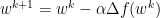
- Outer SGD updates the parameters
- Inner SGD estimates the gradient of local entropy
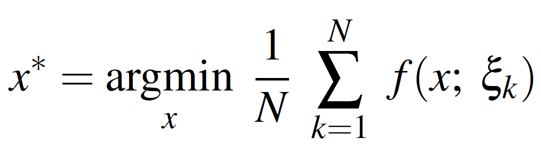
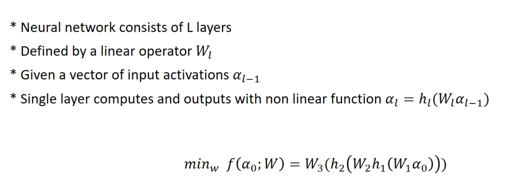
Furthermore the classical (vanilla) optimization problem is like this:
whereas an Entropy-SGD optimization:
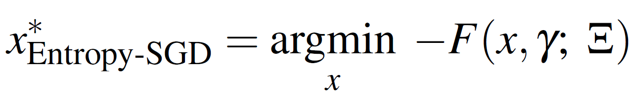 Where Ξ is the data.
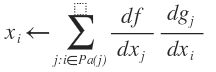
The Gradient of Local Entropy
For  : randomly sampled mini batch of m samples:
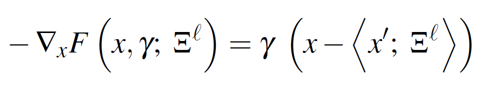
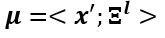
Where for the computation of  the current weights are fixed to x.
Moreover, the Gibbs Distribution of the Original Optimization is:
To this end, they utilize the “Langevin dynamics” (SGLD): an MCMC algorithm. The algorithm is as follows. However, there is a caveat in step 7 that is not properly addressed in the paper.
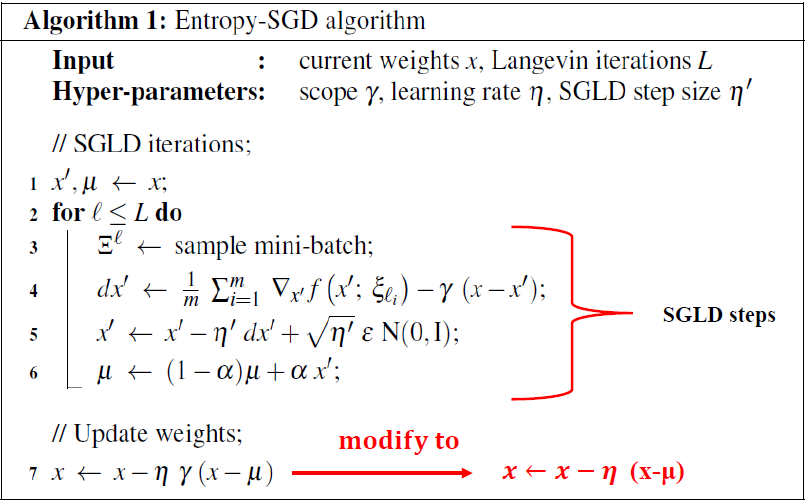
- This algorithm is for 1 iteration:
- ε: thermal noise
- Fix: L, ε, η
- Step 7: As the authors stress, γ has to be tuned (scoping). Thus in practice the algorithm is modified as in Step 7.
The «Scoping» of γ
The scoping is formulated by the following framework:
-
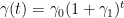
- For
 parameter update
- The General strategy is:
1.Set  very small
2.Large value for η
3.Set  : such that the magnitude of the local entropy is comparable to SGD
THEORETICAL PROPERTIES
The authors show that:
- Entropy-SGD results in a smoother loss function
- and obtains better generalization
With two assumptions:
- The original f(x) is β-smooth
- no eigenvalue of the Hessian ∇^2 f(x) lies in [-2γ-c,c]
- For small c>0

The proof is based on a Laplace Transformation.
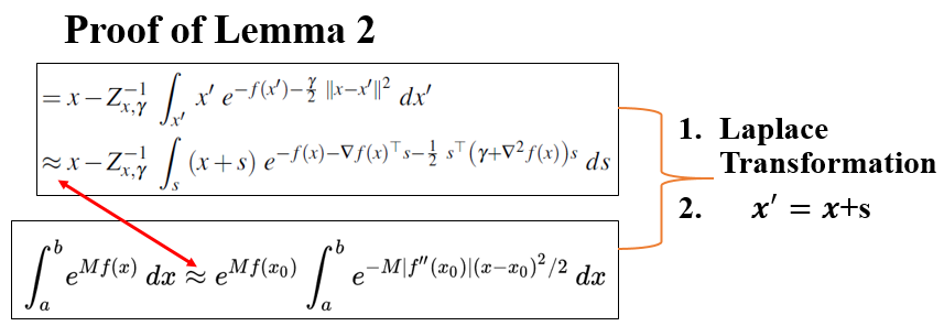
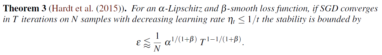
However the assumption regarding the bound is not as strong as the authors suggest. Moreover, the authors cite Hardt et al. (2015) who stress:
“This (assumption) is admittedly unrealistic [..] even if this assumption is violated to an extent before convergence happens.”
The authors are worried about the “stability” of the algorithm. Subsequently, they introduce the concept of an “ε-stable algorithm”, that places an upper bound to the algorithm: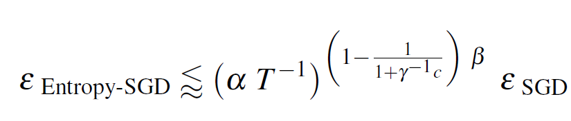
Intuition: Under different samples of the general “population” the algorithm gives the same result, within little changes. The upper bound is derived by Theorem 3 and Lemma 2:
Experiments
The experiments were done as follows:
A. Two image classification datasets
- viz. MNIST
- CIFAR-10
B. Two Text prediction datasets
- viz. PTB
- text of War and Peace
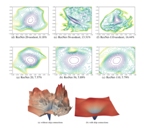
The authors compute the Hessian at a local minimum at the end of training for the following networks:
- small-LeNet on MNIST:
- small-mnistfc on MNIST:
- char-lstm for text generation:
- All-CNN-BN on CIFAR-10
When a Hessian are very close to zero we have an almost flat at local minima. The authors compute the exact Hessian at convergence. The Entropy-SGD model is then compared to the SGD/ADAM. The results are demonstrated in the following Table that reports the the Error/Perplexity(%) per Epoch. The way the following table should be interpreted is that the model that performs better has a lower number of Epochs, for the same Error/Perplexity(%) per Epoch.
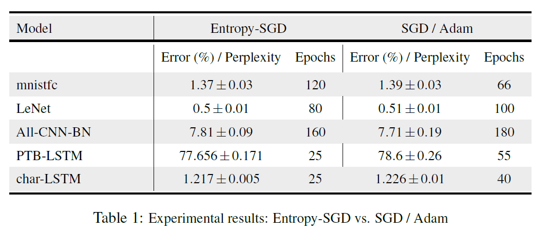
The authors also conducted a comparison between SGLD and Entropy-SGD, which is oddly reported in the Appendix, in the last page of the paper. This comparison was conducted for was for LeNET (300 Epochs) and ALL-CBB-BNN after (500 Epochs). The test error on LeNet of  after 300 epochs and
  on All-CNN-BN after 500 epochs. ARXIV
Assessment
The authors conclude that by using Langevin Dynamics to estimate “local entropy”: “can be done efficiently even for large deep networks using mini-batch updates”. One of the mane problems in the results is that no run-time speeds are reported. It is unclear whether the procedure’s increased computational cost is offset by the faster convergence. In addition, Baldassi et al. 2016 used a method called “Belief Propagation” to also estimate local entropy which is probably not given enough credit in this paper.
Notation
The paper uses Bra–ket notation (or Dirac notation) for probabilities:
https://quantummechanics.ucsd.edu/ph130a/130_notes/node107.html
References
[1] Chaudhari, Pratik; Choromanska, Anna; Soatto, Stefano; LeCun, Yann; Baldassi, Carlo; Borgs, Christian; Chayes, Jennifer; Sagun, Levent; Zecchina, Riccardo. Entropy-SGD: Biasing Gradient Descent Into Wide Valleys. 2017
[2] Baldassi, C. Borgs, J. T. Chayes, A. Ingrosso, C. Lucibello, L. Saglietti, and R. Zecchina. Unreasonable effectiveness of learning neural networks: From accessible states and robust ensembles to basic algorithmicschemes. PNAS, 113(48):E7655–E7662, 2016.
[3] Nitish Shirish Keskar, Dheevatsa Mudigere, Jorge Nocedal, Mikhail Smelyanskiy, Ping Tak Peter Tang. “On Large-Batch Training for Deep Learning: Generalization Gap and Sharp Minima”. CoRR. 2017
[4] Hochreiter and J. Schmidhuber. Flat minima. Neural Computation, 9(1):1–42, 1997.
[6] M. Hardt, B. Recht, and Y. Singer. Train faster, generalize better: Stability of stochastic gradient descent. arXiv:1509.01240, 2015.


 and
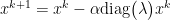
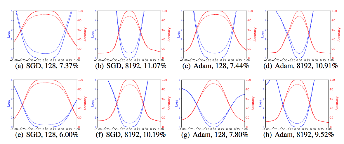
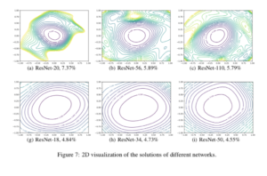
and  , move by certain scale from one point to another along the line connecting these two points and plot the values of the loss function. The points along the line can be computed with a weight parameter
  by
by  .
. , either choose one direction
  to move along and plot a function of the form
  , or choose two directions,
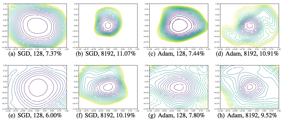
  , plot a 2D surface of the form
  . The 2D plotting is more computationally costly, so the method often produces low-resolution plots of small regions.
 with dimensions compatible with parameter with
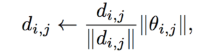
 represents the
  filter (not the jth weight) of the
  layer of
  and
and  respectively. Then they plot 1D interpolation plots between
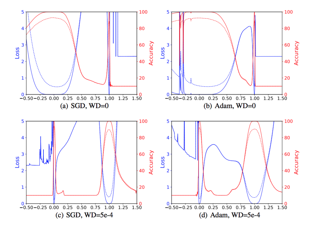
 .
.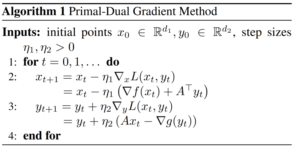


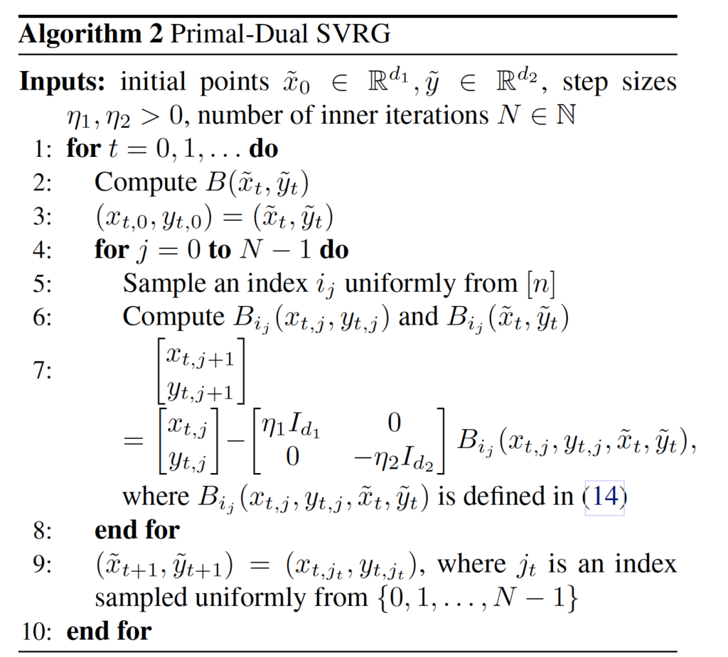
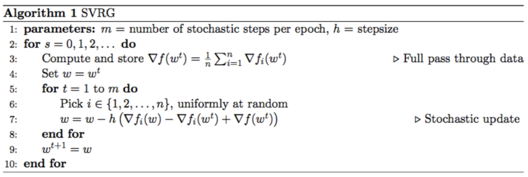
 has full column rank(Section 3). They also extend the primal-dual method to the stochastic situation and propose the primal-dual stochastic variance reduced gradient(SVRG) method. They use the new method to prove that the primal-dual SVRG method also has linear converge rate(Section 4).
 , we can prove that the function satisfies the condition that
  , which implies the linear convergence rate.
 . That is, we want to prove that
  . Second, we bound the decrease of
  . Finally, we prove the inequality.
 , and the relationship between
  and
and  . And then use the triangle inequality to find the relationship among
  ,
,  with the true gradient, i.e.,
  .
.
 and
and  together. In Theorem 4.1, they prove that the primal-dual SVRG also has the linear convergence rate.

 is a finite set of vector that we call atoms. Assume that the function f is
  -strongly convex with L-Lipschitz continuous gradient over M.
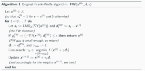
 .
.
 .
.
![f({ x }^{ (t+1) })\le f({ x }^{ (t) })+\gamma <\nabla f({ x }^{ (t) },{ d }_{ t })>+\frac { { \gamma }^{ 2 } }{ 2 } L{ ||{ d }_{ t }|| }^{ 2 }\quad \quad \forall \gamma \in [0,{ \gamma }_{ max }]](https://s0.wp.com/latex.php?latex=f%28%7B+x+%7D%5E%7B+%28t%2B1%29+%7D%29%5Cle+f%28%7B+x+%7D%5E%7B+%28t%29+%7D%29%2B%5Cgamma+%3C%5Cnabla+f%28%7B+x+%7D%5E%7B+%28t%29+%7D%2C%7B+d+%7D_%7B+t+%7D%29%3E%2B%5Cfrac+%7B+%7B+%5Cgamma+%7D%5E%7B+2+%7D+%7D%7B+2+%7D+L%7B+%7C%7C%7B+d+%7D_%7B+t+%7D%7C%7C+%7D%5E%7B+2+%7D%5Cquad+%5Cquad+%5Cforall+%5Cgamma+%5Cin+%5B0%2C%7B+%5Cgamma+%7D_%7B+max+%7D%5D&bg=ffffff&fg=000&s=0&c=20201002) (1)
(1) to minimize RHS:
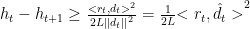 ,when
,when  is big enough.
 -strong convexity of f, we can get (with
  ):
):![f({ x }^{ (t) }+\gamma { e }_{ t })\ge f({ x }^{ (t) })+\gamma <\nabla f({ x }^{ (t) },{ e }_{ t })>+\frac { { \gamma }^{ 2 } }{ 2 } \mu { ||{ e }_{ t }|| }^{ 2 }\quad \forall \gamma \in [0,1]](https://s0.wp.com/latex.php?latex=f%28%7B+x+%7D%5E%7B+%28t%29+%7D%2B%5Cgamma+%7B+e+%7D_%7B+t+%7D%29%5Cge+f%28%7B+x+%7D%5E%7B+%28t%29+%7D%29%2B%5Cgamma+%3C%5Cnabla+f%28%7B+x+%7D%5E%7B+%28t%29+%7D%2C%7B+e+%7D_%7B+t+%7D%29%3E%2B%5Cfrac+%7B+%7B+%5Cgamma+%7D%5E%7B+2+%7D+%7D%7B+2+%7D+%5Cmu+%7B+%7C%7C%7B+e+%7D_%7B+t+%7D%7C%7C+%7D%5E%7B+2+%7D%5Cquad+%5Cforall+%5Cgamma+%5Cin+%5B0%2C1%5D&bg=ffffff&fg=000&s=0&c=20201002)


 i = 1, …, m
 i = 1, …, p
 , domain
  is nonempty. The optimal value is
  .
. as:
as:
 ,
,  as the Lagrange multiplier associated with the
  inequality constraint
  and
and  as the Lagrange multiplier associated with the
  .
.

 , then
  .
. is feasible and
  , then


 , this property is called weak duality. The weak duality inequality holds when
  and
and  are infinite while If the equality
  holds then we say that strong duality holds.
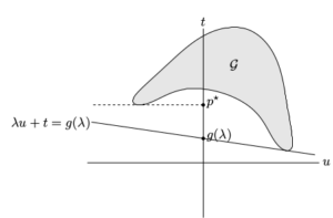
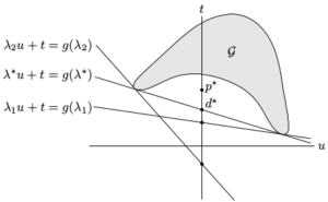
 over
over  . This yields a supporting hyperplane with slope −λ. The intersection of this hyperplane with the u = 0 axis gives g(λ). Supporting hyperplanes corresponding to three dual feasible values of λ, i.e, optimum
  ,
,  , and
, and  . As shown in the figures, strong duality does not hold so the optimal duality gap
  is positive.
 is the profit made at the operating condition x.
 represents some limit on resources (e.g., warehouse space, labor) or a regulatory limit (e.g., environmental). The operating condition that maximizes profit while respecting the limits can be found by solving the problem:
 resulting optimal profit is
  . Enterprise for the
  limit or constraint is
  . Payments are also made to the firm for constraints that are not tight; if
  has the interpretation of the price for violating
  , i.e., the firm must pay for violations.

 Comparing to the existing work on GPU, this paper can train ResNet-50 on ImageNet to get 76.1% accuracy in 30 mins, by making the full use of the characteristic of TPU.
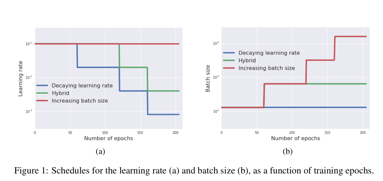 Figure 1 shows an example that how the learning rate and batch size change in the different algorithms. For the blue line decaying learning rate, the learning rate is reduced in the training process (number of epochs increase) but the batch size is always constant. For the red line increasing batch size, the batch size is increased in the training process (number of epochs increase) but the learning rate is always constant.
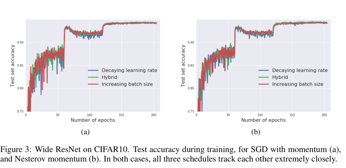
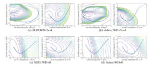
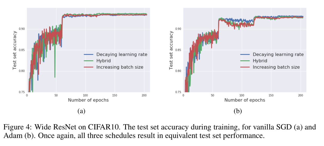 Figure 3 and Figure 4 show that the batch size increasing approach can be applied to many different optimization algorithms, like SGD with momentum, Newterow momentum, vanilla SGD and Adam.
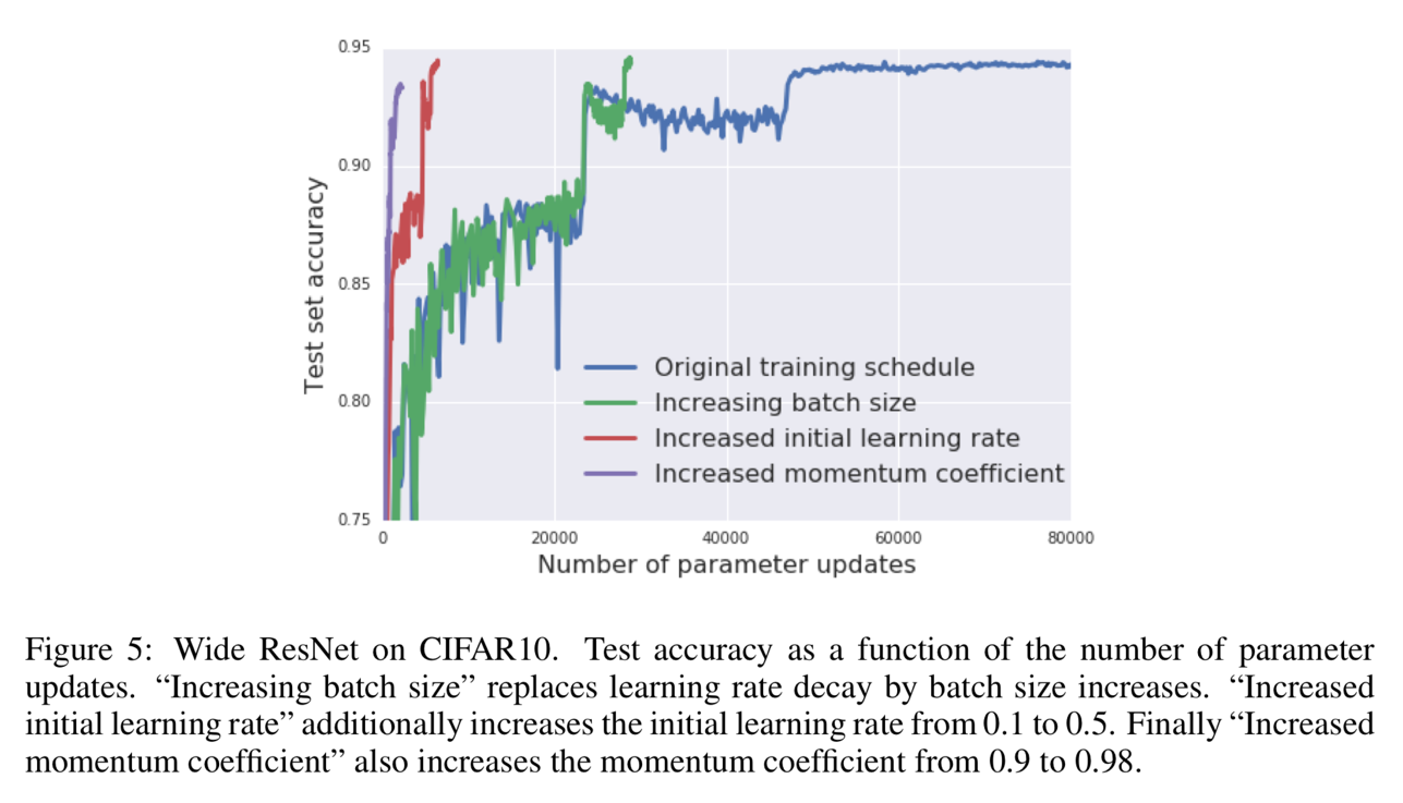
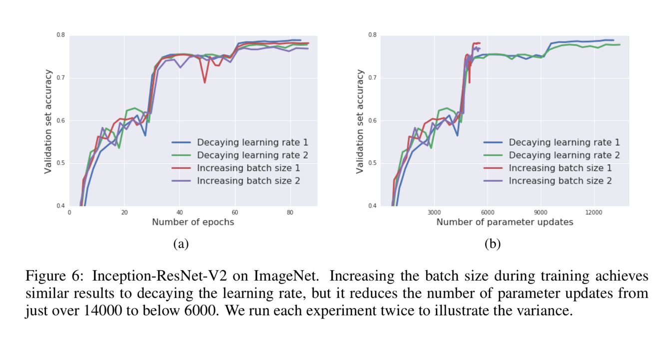 Figure 6 proves the validity and reproducibility of this algorithm by conducting the experiments many times.
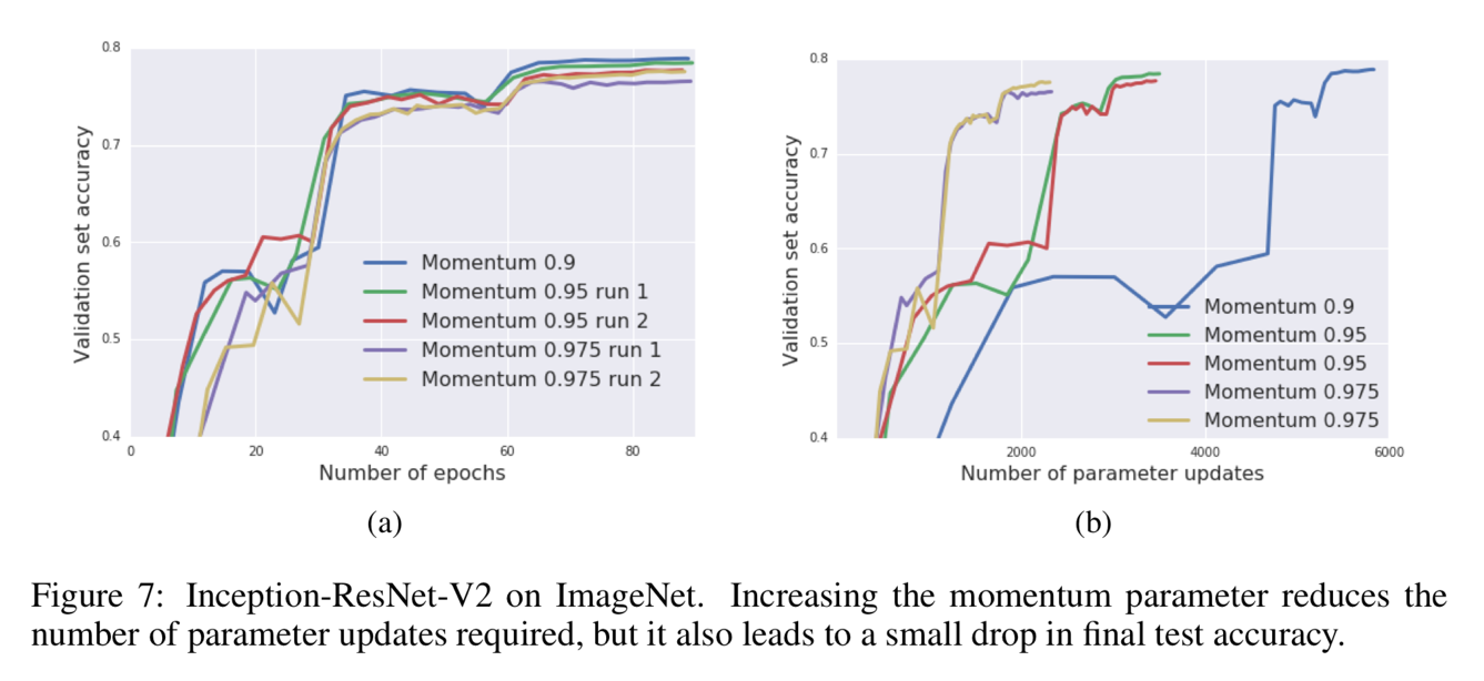 Figure 7 shows that the influence of momentum coefficient that increasing the momentum can reduce the update times as well as reduce the training time consuming but can let the accuracy fall a little bit.
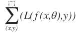

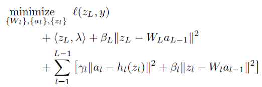
 objective function is shown as above.
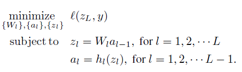

 then
then