1. Lagrange dual problem: standard form, Lagrange dual function, and dual problem
First, we consider an optimization problem in the standard form:
minimize 
subject to  i = 1, …, m
 i = 1, …, p
with variable  , domain
  is nonempty. The optimal value is
  .
.
The idea of lagrangian duality is to take the constraints into account by augmenting the objective function with a weighted sum of the constraint functions.
Lagrangian  as:
as:

with  ,
,  as the Lagrange multiplier associated with the
  inequality constraint
  and
and  as the Lagrange multiplier associated with the equality constraint
  .
.
Lagrange dual function is the minimum value of the Lagrangian.
For 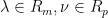

If  , then
  .
.
Proof:
If  is feasible and
  , then

minimizing over all feasible gives 
The dual problem: what is the best lower bound that can be obtained from the Lagrange dual function?
maximize 
subject to
Optimal value is denoted as 
2. Weak and strong duality
If  , this property is called weak duality. The weak duality inequality holds when
  and
and  are infinite while If the equality
  holds then we say that strong duality holds.
3. Geometric interpretation of dual function and lower bound 
For a problem with one (inequality) constraint. Given λ, we minimize  over
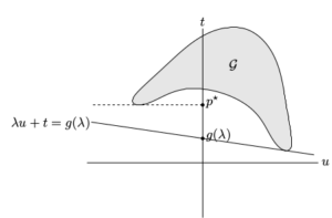
over  . This yields a supporting hyperplane with slope −λ. The intersection of this hyperplane with the u = 0 axis gives g(λ). Supporting hyperplanes corresponding to three dual feasible values of λ, i.e, optimum
  ,
,  , and
, and  . As shown in the figures, strong duality does not hold so the optimal duality gap
  is positive.
4. Price or profit interpretation
Suppose the variable x denotes how an enterprise operates and denotes the cost of operating at x, then  is the profit made at the operating condition x.
Each constraint  represents some limit on resources (e.g., warehouse space, labor) or a regulatory limit (e.g., environmental). The operating condition that maximizes profit while respecting the limits can be found by solving the problem:
minimize 
subject to , i = 1, …, m.
The resulting optimal profit is  resulting optimal profit is .
Now imagine a second scenario in which the limits can be violated, by paying an additional cost which is linear in the amount of violation, measured by  . Enterprise for the
  limit or constraint is
  . Payments are also made to the firm for constraints that are not tight; if represents a payment to the firm.
The coefficient  has the interpretation of the price for violating ; its units are dollars per unit violation. For the same price the enterprise can sell any ‘unused’ portion of the constraint. We assume
  , i.e., the firm must pay for violations.
Reference
Boyd and Vandenberghe, Chapter 5–5.5 https://web.stanford.edu/~boyd/cvxbook/bv_cvxbook.pdf