On the Global Linear Convergence of Frank-Wolfe Optimization Variants

1.Introduction

The Frank-Wolfe (FW) optimization algorithm has lately regained popularity thanks in particular to its ability to nicely handle the structured constraints appearing in machine learning applications.

In this section, consider the general constrained convex problem of the form:

$\underset { x\in M }{ min } f(x),\quad M=conv(A),\quad with\quad only\quad access\quad to:\quad { LMO }_{ A }(r)\in \underset { x\in A }{ arg min } <r,x>$

Where $A\subseteq { R }^{ d }$ is a finite set of vector that we call atoms. Assume that the function f is $\mu$ -strongly convex with L-Lipschitz continuous gradient over M.

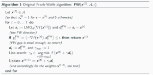
2. Original Frank-Wolfe algorithm

The Frank-Wolfe (FW) optimization algorithm, also known as conditional gradient, is particularly suited for the setup. It works as follows:

At a current iterate x^(t), the algorithm finds a feasible search atom st to move towards by minimizing the linearization of the objective function f over M – this is where the linear minimization oracle LMOa is used.

The next iterate x^(t+1) is then obtained by doing a line-search on f between x^(t) and st.

3. Variants of Frank-Wolfe algorithm

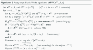
3.1 Away-Frank-Wolfe Algorithm

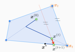
However, there is zig-zagging phenomenon. In order to address this phenomenon, away-Frank-Wolfe algorithm is proposed. Add the possibility to move away from an active atom in ${ S }^{ (t) }$ .

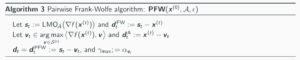
3.2 Pairwise Frank-Wolfe Algorithm

pairwise Frank-Wolfe algorithm is also called MDM algorithm. At first, it proposed to address the polytope distance problem. It hopes to move weight mass between two atoms in each step. According to the algorithm 3, we can know that is almost algorithm 2, except ${ d }_{ t }={ { d }_{ t } }^{ PFW }:={ s }_{ t }-{ v }_{ t }\quad and\quad { \gamma }_{ max }:={ \alpha }_{ { v }_{ t } }$ .

4. Global Linear Convergence Analysis

In this paper, section 2 is talking about global linear convergence analysis. We can see that at first, it introduce the proof elements and convergence proof. And lately, section 2.2 is talking convergence results.

4.1 proof of convergence

4.1.1

As f has the L-Lipschitz gradient, we can get

$f({ x }^{ (t+1) })\le f({ x }^{ (t) })+\gamma <\nabla f({ x }^{ (t) },{ d }_{ t })>+\frac { { \gamma }^{ 2 } }{ 2 } L{ ||{ d }_{ t }|| }^{ 2 }\quad \quad \forall \gamma \in [0,{ \gamma }_{ max }]$ (1)

Choose $\gamma$ to minimize RHS:

${ h }_{ t }-{ h }_{ t+1 }\ge \frac { { <{ r }_{ t },{ d }_{ t }> }^{ 2 } }{ 2L{ ||{ d }_{ t }|| }^{ 2 } } =\frac { 1 }{ 2L } { <{ r }_{ t },{ \hat { d } }_{ t }> }^{ 2 }$ ,when ${ \gamma }_{ max }$ is big enough.

4.1.2

By $\mu$ -strong convexity of f, we can get (with ${ e }_{ t }:={ x }^{ * }-{ x }^{ (t) }$ ):

$f({ x }^{ (t) }+\gamma { e }_{ t })\ge f({ x }^{ (t) })+\gamma <\nabla f({ x }^{ (t) },{ e }_{ t })>+\frac { { \gamma }^{ 2 } }{ 2 } \mu { ||{ e }_{ t }|| }^{ 2 }\quad \forall \gamma \in [0,1]$

Use $\gamma$ =1 on LHS get:

${ h }_{ t }\le \frac { { { <r }_{ t },{ \hat { e } }_{ t }> }^{ 2 } }{ 2\mu }$

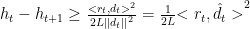
4.1.3

combining 4.1.1 and 4.1.2, we can get

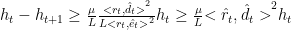
${ h }_{ t }-{ h }_{ t+1 }\ge \frac { \mu }{ L } \frac { { { <r }_{ t },{ \hat { d } }_{ t }> }^{ 2 } }{ L{ <{ r }_{ t },{ \hat { e } }_{ t }> }^{ 2 } } { h }_{ t }\ge \frac { \mu }{ L } { <{ \hat { r } }_{ t },{ \hat { d } }_{ t }> }^{ 2 }{ h }_{ t }$

Thus, lower bounds * to get linear convergence rate.

5. Conclusion

This paper reviews variant of FW algorithm and shows for the first time global linear convergence for all variants of FW algorithm. It introduces of the notion of the condition number of the constraint set.

6. Reference

1. Simon Lacoste- Julien & Martin Jaggi: On the global linear convergence of Frank-Wolfe optimization variants.

2. Simon Lacoste- Julien & Martin Jaggi: http://www.m8j.net/math/poster-NIPS2015-AFW.pdf

3. R. Denhardt-Eriksson & F. Statti: http://transp-or.epfl.ch/zinal/2018/slides/FWvariants.pdf

Leave a Reply Cancel reply