Subgradient Method
Subgradient method is the basic optimization algorithm for convex nondifferentiable functions. First, let’s see what a subgradient is. A subgradient is a generalization of the gradient for nondifferentiable functions. For simplicity, let’s elaborate it in a one-dimensional space. The gradient of a function at a certain point is the slope of the tangent line at that point.
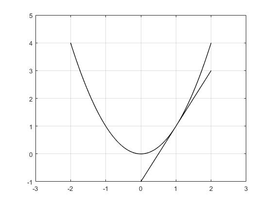
However, for nondifferentiable functions, there is no unique gradient at nondifferentiable points. Instead, there are subgradients 
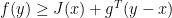
All vectors
In Fig. 2, you can see that slopes of both blue and red lines are subgradients of the function at 
Now assume that our goal is to minimize the cost function 
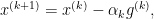
where 

However, the subgradient direction is not always a descent direction (can you think of an example?), so we have to keep track of the smallest objective function value that we have reached so far(i.e. iteration 

The proof of convergence for this algorithm depends on three conditions:
- The function
- The size of the subgradient is bounded, i.e,
for all
- The distance of the initial point to the optimal set is bounded by
, i.e.,
.
With the aforementioned conditions, it is shown that the distance between best point found so far 

Now, depending on the step size 
- Constant step size
: which is a positive constant. In this case, we will have
. As
.
- Square summable but not summable
,

We showed that the convergence rate in both cases are sublinear with the definition here.
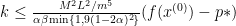
Also, we discussed in class that if the number of iterations is determined, i.e., we want to reach the best we can in

Using this bound, we found that if we want to reduce the gap between the current objective value and the optimal objective by a factor of 1000, we need 

Stochastic Gradient Descent
We have seen that we can use standard gradient descent given a convex function and its gradient. We discussed earlier in this section that we can use subgradient descent given a convex function with undefined gradient and its subgradient. What approach is appropriate when we are given a convex function with a stochastic gradient?
Stochastic gradient descent (SGD) is a term used to describe the application of classic gradient descent and subgradient methods when only a stochastic estimate of the true (sub)gradient is available.
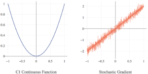
To get a better feel for what this means and why this is useful, imagine the following two motivating examples. First, consider the training of a neural network (NN) when we have millions of training samples. The huge number of training samples causes the calculation of the gradient to be very expensive, making training slow. We could randomly select a subset of training samples (say, 1000 of them) and compute a gradient with respect to only that sample. We assume (and in this case, know) that the gradient estimate generated from a sample will behave like the true gradient on average and still point us in a general descent direction.
In another example consider a black box optimization problem, meaning that the optimization algorithm only has access to actual function values *without* gradient information. At first glance, it may seem like gradient descent methods cannot be used for this problem. However, if we assume that the underlying function has some amount of “smoothness” and randomly sample function values near the current iterate, we can use a least squares fit to estimate the gradient.
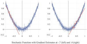
In general, the formal assumption for any SGD method is that the optimization algorithm has access to an estimate 


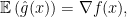
where 
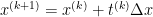
Using

where 
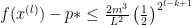
We see two convergence proofs for this vanilla SGD. The first leverages an inductive argument to show that for a strongly convex differentiable function $f$, after 


where 
In a slight modification, often called “robust” SGD, we relax the assumptions so that 


 .
. for which
 ,
, such that
 .
. ,
, is considered a constant, and
  is the value of
  ,
, .
. ,
, .
. and
and  , and the secant condition is
 .
.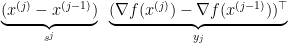 ,
, and
and  are the shorthand used to describe these difference vectors in the slides. Based on the existence of these outer products, it appears as if an
  cost is unavoidable, when all the literature says the memory and running time costs are
  .
. . We then have products of length-
 ,
, .
.