Momentum adds a relatively subtle change to gradient descent by replace f with z. Where
As such, alpha retains the role of representing the step size. However, we introduce a new constant, beta. Beta adds a decaying effect on momentum, and must be between 0 and 1, noninclusive. We briefly demonstrate the edge cases of beta below:
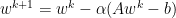
We now introduce a change of basis which will be convenient for later. Consider a matrix form of gradient descent:
Which has optimal solution
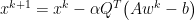
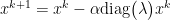
we consider the eigenvectors of A which is a natural space of viewing A where all dimensions act independently.
Thus, we now can view gradient descent in basis of the eigenvectors of A. We consider the contributions of error as
$latex f(w^k)-f(w^\star) = \sum (1 – \alpha \lambda_i)^{2k} \lambda_i [x_i^0]^2 $
For convergence, we note that
$latex 1 – \alpha \lambda_i $
must be strictly less than 1.
The performance of Neural Networks could be affected by the landscape of loss function, which is decided by a wide range of factors including network architecture, the choice of optimizer, variable initialization, etc. Studying and visualizing the effect of these factors on the underlying loss landscape is challenging because they often lie in high-dimensional spaces and are hard to be captured geometrically, while human perceivable visualizations are only low-dimensional 1D (line) or 2D (surface) plots. The paper we read is therefore motivated to close this dimensionality gap and proposes visualization method that can enable meaningful side-by-side comparisons.
Basics
Given input data (feature vectors {xi} and accompanying labels {yi}), neural network losses are high-dimensional non-convex functions computed with the parameter set \theta. The paper first reviews two conventional method to visualize the loss landscape:
1-Dimensional Linear Interpolation
Choose two sets of parameters and , move by certain scale from one point to another along the line connecting these two points and plot the values of the loss function. The points along the line can be computed with a weight parameter by .
2D Contour Plots
Choose a center point , either choose one direction to move along and plot a function of the form , or choose two directions, and , plot a 2D surface of the form . The 2D plotting is more computationally costly, so the method often produces low-resolution plots of small regions.
Filter Normalization
Scale Invariance
When random directions are used in visualization, the plots are sensitive to the scale of model weights. “A neural network with large weights may appear to have a smooth and slowly varying loss function”. However, neural networks are scale invariant, especially when batch normalization is applied to rescale the output of each layer.
Filter Normalization
In order to remove the scaling effect and enable meaningful comparisons between plots, the paper proposes to use filter-wise normalized directions. Given a random Gaussian direction with dimensions compatible with parameter with , each filter in is normalized to have the same norm of the corresponding filter in :
where represents the filter (not the jth weight) of the layer of .
The Sharp vs. Flat Delemma
The authors then applied filter normalized directions to study whether sharp minimizers generalize better than flat minimizers. It is widely believed that small-batch SGD usually produces “flat” minimizers while large batch sizes produce “sharp” minima with poor generalization”, so they train a CIFAR-10 classifier using a 9-layer VGG network, running SGD with small batches and large batches produces solution and respectively. Then they plot 1D interpolation plots between and . However, as shown in the figure below, with these plots, there is no apparent correlation between sharpness and generalization because it can easily flipped by turning on a small weight decay.
The flipping is because adding weight decay reduces the scale of weights, small weights are more sensitive to perturbation and therefore produce sharper looking minimizers.
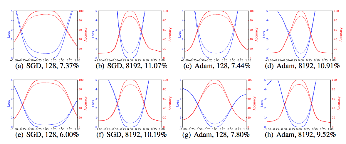
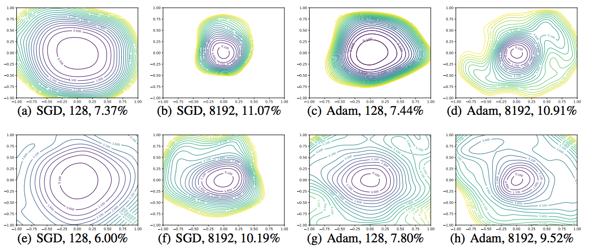
Then they apply filter normalized directions to make 1D and 2D plots. These plots remove the effect of the scale of weights, and from the results, we can make meaningful side-by-side comparisons and conclude that large batches do produce sharper minima with higher test error.
Skip Connections and Dropout
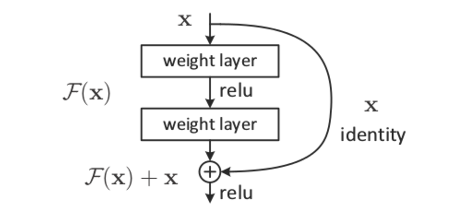
This paper mentions skip connections, which is a method commonly used in very deep networks in order to preserve the values of the input batches through the decay caused by the vanishing gradient problem. In essence, the output of some layers are directly inputted into layer much further down in the network, networks which utilize this are called Residual networks and are the basis for the current SOTA on images. This method is different from dropout, which gives a probability for certain neurons in a network to just output zero no matter their inputs. Both of these methods supposedly help a network in generalization, but there are no real mathematical justifcations for either – just experiments which show networks performing better when using these techniques.
Skip Connections
This paper attempts to show that the practical affects of adding these methods are actually realted to the loss surface of the network. They increase the overall convexity of the surface and have a smoothing effect, which means that the random initalization of the weights has a higher probability to be in an “escapeable” region of the loss surface that will converge to a local minima.
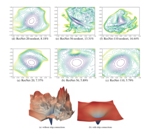
“For the more shallow networks (ResNet-20 and ResNet-20-noshort), the effect of skip connections is fairly unnoticeable. However residual connections prevent the explosion of non-convexity that occurs when networks get deep.”
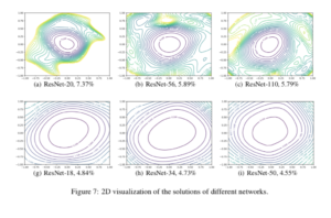
Wide vs. Thin Models
“Increased network width resulted in flat minima and wide regions of apparent convexity”
In this figure, Resnet 18/34/50 contain more convolutional filters per layer than Resnet 20/56/110 and are also shallower, which means less inherent non-convexity according to this paper
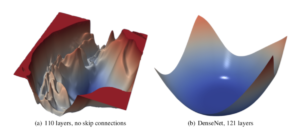
Depth causes non-convexity
As network depth increases, this paper notes that “VGG-like” (or very deep networks without residual connections) transition from nearly convex to chaotic loss surfaces. This chaos also has a effect on the sharpness of the minima of the loss surface, where these chaotic surfaces have much sharper minima and the counters near these are perturbed as well so that optimization is doubly difficult. However, by simply adding residual (skip) connections in the very deep network, this effect is easily reversed.
Optimization Paths
In high dimensional space, two randomly chosen vectors have a very high chance to be nearly orthogonal, meaning that this is very little variance between them. Therefore this paper uses PCA in order to carefully choose two vectors to show descent on, which is especially useful if the descent path is in very low dimensions. The authors of this paper make the claim that 40-90% of variation in the descent path lies in only two dimensions, which means using those two dimensions to produce the optimization path will result in nicely visually descent towards a convex attractor.
Conclusion
Quite a bit of discussion towards the end of our presentation was around the actual helpfulness of visualization methods, and whether using other statistical measures would provide for more information to anyone trying to learn about a network or problem.
Our hesitant conclusion was that visualization itself is a sort of statistical measure which can be used to represent a bunch of smaller measures like convexity, average etc. but for troubleshooting a network it probably isn’t very useful. These techniques are more readily used to quickly convey these overall statistical measures during a presentation or to show quick comparisons of networks to possibly show progression in design. At the very least, these visualizations provide some sort of insight into dropout and residual connections which are currently used in the industry because they work without any real mathematical justification.
The convex-concave saddle point problem has the following format:
For many machine learning applications, their objective functions can be written in the convex-concave format. The example applications include reinforcement learning, empirical risk minimization and robust optimization etc.
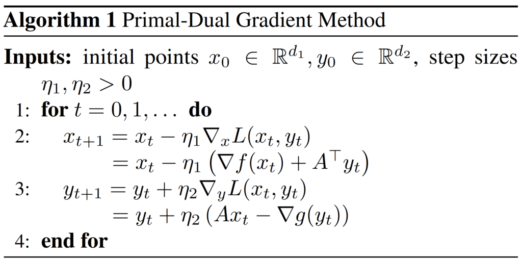
We can use the following primal-dual gradient method to optimize the .
In this paper, the authors develop a new method to prove that the primal-dual gradient method has linear convergence rate, when the and are smooth, is convex, is strongly convex and the coupling matrix has full column rank(Section 3). They also extend the primal-dual method to the stochastic situation and propose the primal-dual stochastic variance reduced gradient(SVRG) method. They use the new method to prove that the primal-dual SVRG method also has linear converge rate(Section 4).
Preliminaries
Before we prove the convergence of the primal-dual method, we need some preliminaries. First, we need the definitions of smoothness and strong convexity.
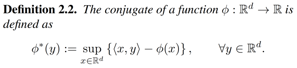
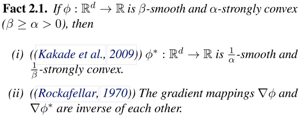
We also need the definition and some properties of the conjugate function.
Based on the definition of conjugate function, we can get the corresponding primal problem of the .
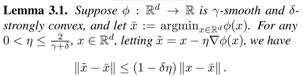
Finally, we need the of gradient descent on the strongly convex function.
Linear Convergence of the Primal-Dual Gradient Method
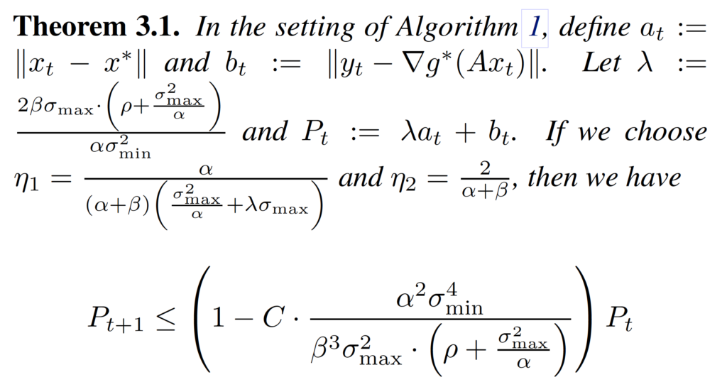
With these preliminaries, we can start to prove the convergence of primal-dual gradient method. The Theorem 3.1 establishes the linear convergence guarantee for it.
This theorem says that if we construct a Lyapunov function , we can prove that the function satisfies the condition that , which implies the linear convergence rate.
We can divide the proof of this theorem to three steps. First, we bound the decrease of . That is, we want to prove that . Second, we bound the decrease of . Finally, we prove the inequality.
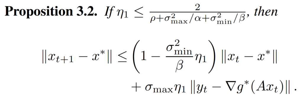
Proposition 3.1 and Proposition 3.2 give the bound of decrease of .
The proof technique of the first step is to first find the relationship between and , and the relationship between and . And then use the triangle inequality to find the relationship among , and . The authors call the ghost variable in this paper, which is actually the $x$ obtained by updating the with the true gradient, i.e., .
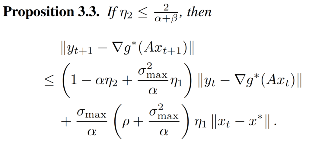
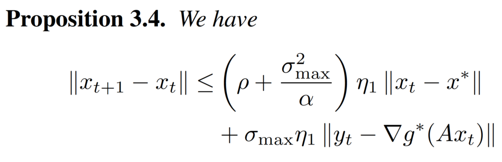
Proposition 3.3 and Proposition 3.4 give the bound of decrease of . We can use the convex function’s property to prove them.
After we have these propositions, we can put them together, and with some routine calculations, we can prove the inequality in Theorem 3.1.
Extension to the Primal-Dual Stochastic Variance Reduced Gradient Method
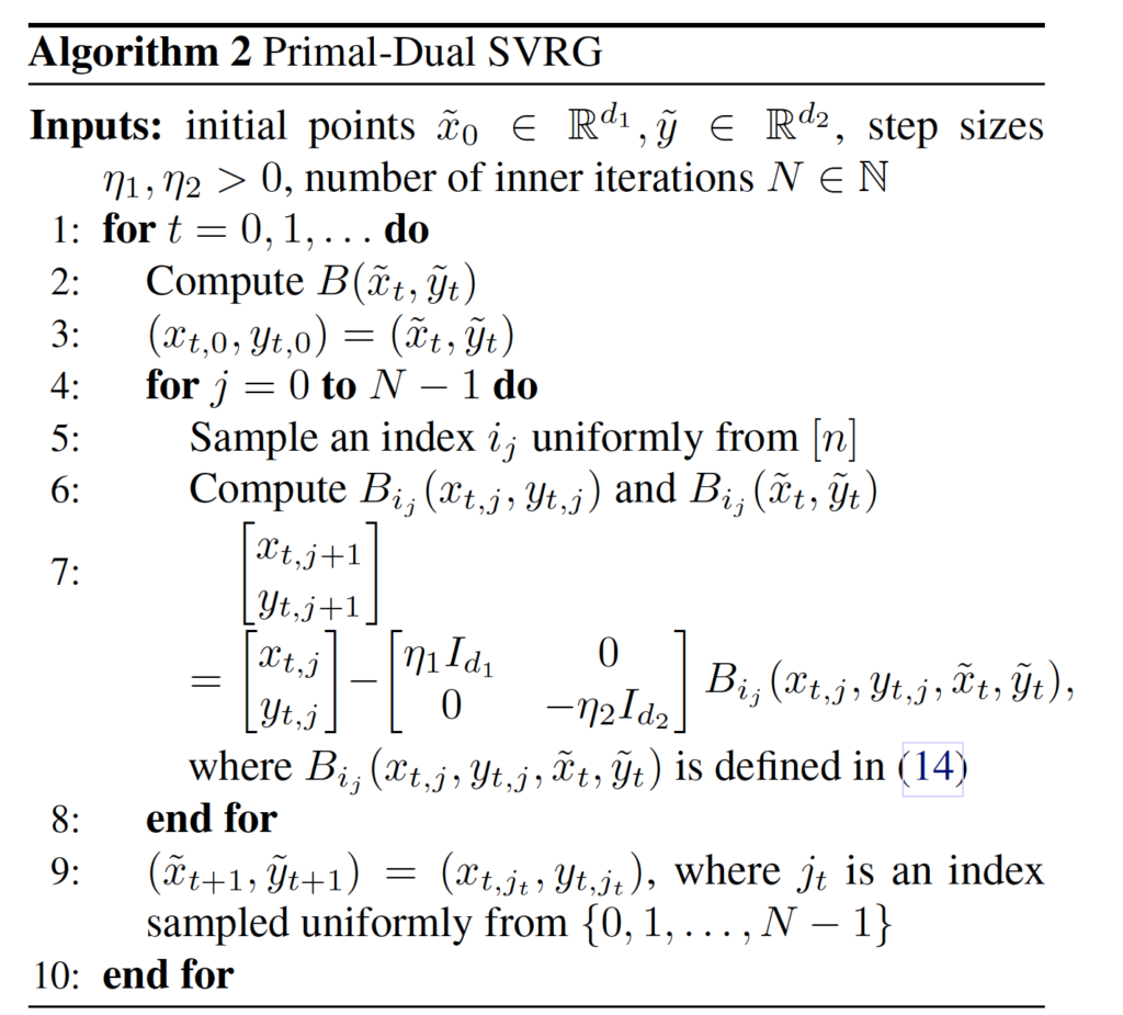
In this section, the authors propose the primal-dual SVRG, and prove its convergence using the same proof method in the third section. The primal-dual SVRG is in Algorithm 2.
The framework of primal-dual SVRG is the same as the vanilla SVRG. The main difference is only that the primal-dual SVRG updates the parameters and together. In Theorem 4.1, they prove that the primal-dual SVRG also has the linear convergence rate.
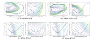
Preliminary Empirical Evaluation
They do experiments on synthetic dataset to prove the convergence of primal-dual gradient method. The results are as below.
The Frank-Wolfe (FW) optimization algorithm has lately regained popularity thanks in particular to its ability to nicely handle the structured constraints appearing in machine learning applications.
In this section, consider the general constrained convex problem of the form:
Where is a finite set of vector that we call atoms. Assume that the function f is -strongly convex with L-Lipschitz continuous gradient over M.
2. Original Frank-Wolfe algorithm
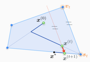
The Frank-Wolfe (FW) optimization algorithm, also known as conditional gradient, is particularly suited for the setup. It works as follows:
At a current iterate x^(t), the algorithm finds a feasible search atom st to move towards by minimizing the linearization of the objective function f over M – this is where the linear minimization oracle LMOa is used.
The next iterate x^(t+1) is then obtained by doing a line-search on f between x^(t) and st.
3. Variants of Frank-Wolfe algorithm
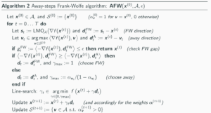
3.1 Away-Frank-Wolfe Algorithm
However, there is zig-zagging phenomenon. In order to address this phenomenon, away-Frank-Wolfe algorithm is proposed. Add the possibility to move away from an active atom in .
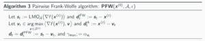
3.2 Pairwise Frank-Wolfe Algorithm
pairwise Frank-Wolfe algorithm is also called MDM algorithm. At first, it proposed to address the polytope distance problem. It hopes to move weight mass between two atoms in each step. According to the algorithm 3, we can know that is almost algorithm 2, except .
4. Global Linear Convergence Analysis
In this paper, section 2 is talking about global linear convergence analysis. We can see that at first, it introduce the proof elements and convergence proof. And lately, section 2.2 is talking convergence results.
4.1 proof of convergence
4.1.1
As f has the L-Lipschitz gradient, we can get
(1)
Choose to minimize RHS:
,when is big enough.
4.1.2
By -strong convexity of f, we can get (with ):
Use =1 on LHS get:
4.1.3
combining 4.1.1 and 4.1.2, we can get
Thus, lower bounds * to get linear convergence rate.
5. Conclusion
This paper reviews variant of FW algorithm and shows for the first time global linear convergence for all variants of FW algorithm. It introduces of the notion of the condition number of the constraint set.
6. Reference
1. Simon Lacoste- Julien & Martin Jaggi: On the global linear convergence of Frank-Wolfe optimization variants.
2. Simon Lacoste- Julien & Martin Jaggi: http://www.m8j.net/math/poster-NIPS2015-AFW.pdf
3. R. Denhardt-Eriksson & F. Statti: http://transp-or.epfl.ch/zinal/2018/slides/FWvariants.pdf


 and
and  , move by certain scale from one point to another along the line connecting these two points and plot the values of the loss function. The points along the line can be computed with a weight parameter
  by
by  .
. , either choose one direction
  to move along and plot a function of the form
  , or choose two directions,
  , plot a 2D surface of the form
  . The 2D plotting is more computationally costly, so the method often produces low-resolution plots of small regions.
 with dimensions compatible with parameter with
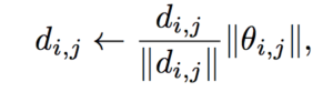
 represents the
  filter (not the jth weight) of the
  layer of
  and
and  respectively. Then they plot 1D interpolation plots between
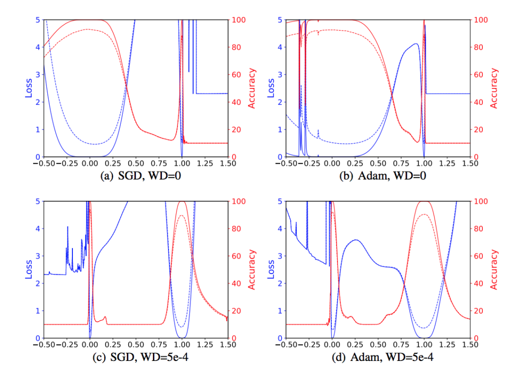
 .
.


 has full column rank(Section 3). They also extend the primal-dual method to the stochastic situation and propose the primal-dual stochastic variance reduced gradient(SVRG) method. They use the new method to prove that the primal-dual SVRG method also has linear converge rate(Section 4).
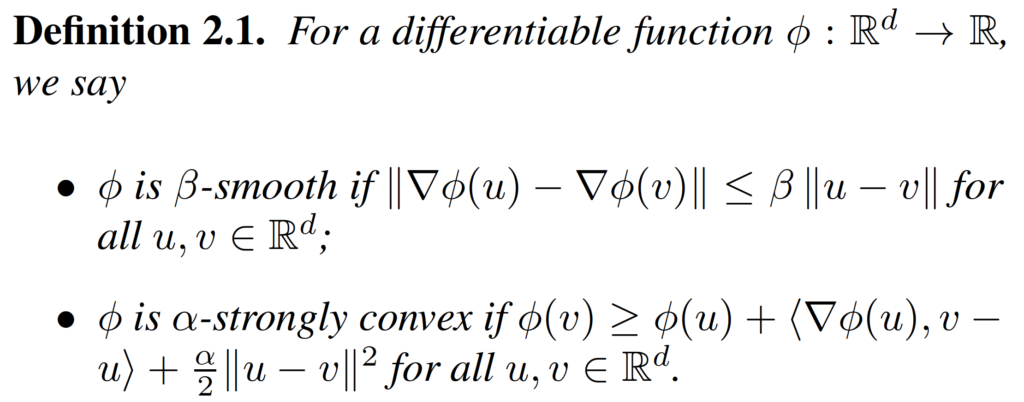
 , we can prove that the function satisfies the condition that
  , which implies the linear convergence rate.
 . That is, we want to prove that
  . Second, we bound the decrease of
  . Finally, we prove the inequality.
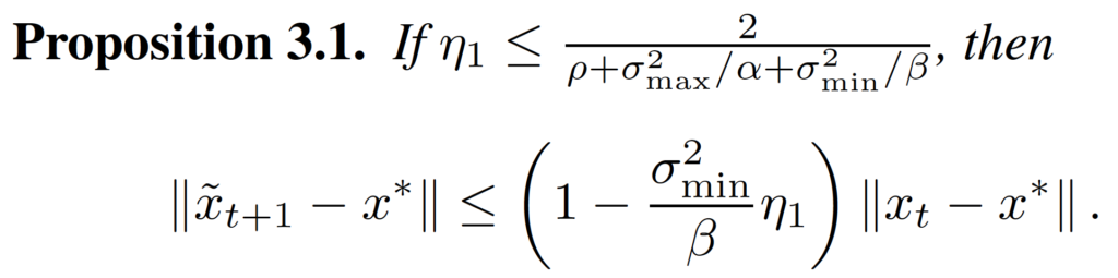
 , and the relationship between
  and
and  . And then use the triangle inequality to find the relationship among
  ,
,  with the true gradient, i.e.,
  .
.
 and
and  together. In Theorem 4.1, they prove that the primal-dual SVRG also has the linear convergence rate.
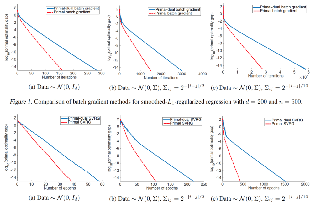

 is a finite set of vector that we call atoms. Assume that the function f is
  -strongly convex with L-Lipschitz continuous gradient over M.
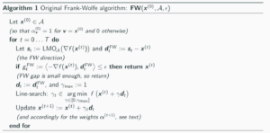
 .
.
 .
.
![f({ x }^{ (t+1) })\le f({ x }^{ (t) })+\gamma <\nabla f({ x }^{ (t) },{ d }_{ t })>+\frac { { \gamma }^{ 2 } }{ 2 } L{ ||{ d }_{ t }|| }^{ 2 }\quad \quad \forall \gamma \in [0,{ \gamma }_{ max }]](https://s0.wp.com/latex.php?latex=f%28%7B+x+%7D%5E%7B+%28t%2B1%29+%7D%29%5Cle+f%28%7B+x+%7D%5E%7B+%28t%29+%7D%29%2B%5Cgamma+%3C%5Cnabla+f%28%7B+x+%7D%5E%7B+%28t%29+%7D%2C%7B+d+%7D_%7B+t+%7D%29%3E%2B%5Cfrac+%7B+%7B+%5Cgamma+%7D%5E%7B+2+%7D+%7D%7B+2+%7D+L%7B+%7C%7C%7B+d+%7D_%7B+t+%7D%7C%7C+%7D%5E%7B+2+%7D%5Cquad+%5Cquad+%5Cforall+%5Cgamma+%5Cin+%5B0%2C%7B+%5Cgamma+%7D_%7B+max+%7D%5D&bg=ffffff&fg=000&s=0&c=20201002) (1)
(1) to minimize RHS:
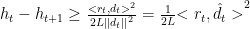 ,when
,when  is big enough.
 -strong convexity of f, we can get (with
  ):
):![f({ x }^{ (t) }+\gamma { e }_{ t })\ge f({ x }^{ (t) })+\gamma <\nabla f({ x }^{ (t) },{ e }_{ t })>+\frac { { \gamma }^{ 2 } }{ 2 } \mu { ||{ e }_{ t }|| }^{ 2 }\quad \forall \gamma \in [0,1]](https://s0.wp.com/latex.php?latex=f%28%7B+x+%7D%5E%7B+%28t%29+%7D%2B%5Cgamma+%7B+e+%7D_%7B+t+%7D%29%5Cge+f%28%7B+x+%7D%5E%7B+%28t%29+%7D%29%2B%5Cgamma+%3C%5Cnabla+f%28%7B+x+%7D%5E%7B+%28t%29+%7D%2C%7B+e+%7D_%7B+t+%7D%29%3E%2B%5Cfrac+%7B+%7B+%5Cgamma+%7D%5E%7B+2+%7D+%7D%7B+2+%7D+%5Cmu+%7B+%7C%7C%7B+e+%7D_%7B+t+%7D%7C%7C+%7D%5E%7B+2+%7D%5Cquad+%5Cforall+%5Cgamma+%5Cin+%5B0%2C1%5D&bg=ffffff&fg=000&s=0&c=20201002)