Training Neural Networks Without Gradients : A Scalable ADMM Approach
Introduction
Many research have been conducted in training Neural Networks. Most common method is using stochastic gradient method combine with backpropagation. The paper notice the weakness of this conventional method and suggest their proposed method which is using alternating direction method of multipliers (ADMM) with bregman iteration.
Why we need proposed method ?
Weakness of conventional optimization rely on stochastic gradient method in Neural Networks is that they do not scale well to large number of cores in a cluster setting. Also as the method is gradient-based, there are problems with convergence such as saturation effect or stock in local optimal point or vanishing gradients. In addition, backpropagation does not easily parallelize over layers.
To solve these problems proposed method separate the objective function at each layer of a neural network into two terms.
First term is measuring the relation between the weights and the input activations. Second term is containing the nonlinear activation function.
This structure allows the weights to be updated without the effects of vanishing gradient and stock in local optimal. Also form of the objective allows the weights of every layer to be updated independently, enabling parallelization over layers.
By separating the objective function, proposed method decomposes with the sequence of minimization sub problems which is ADMM scheme, and it can solve globally & closed form. Also, combining bregman iteration, the solution of proposed method could be stable.
In addition proposed method exhibits linear scaling when data is parallelized across cores.
Notation
Let’s define notation, before checking the model of proposed method.
Neural network consists of L layers and defined by a linear operator W
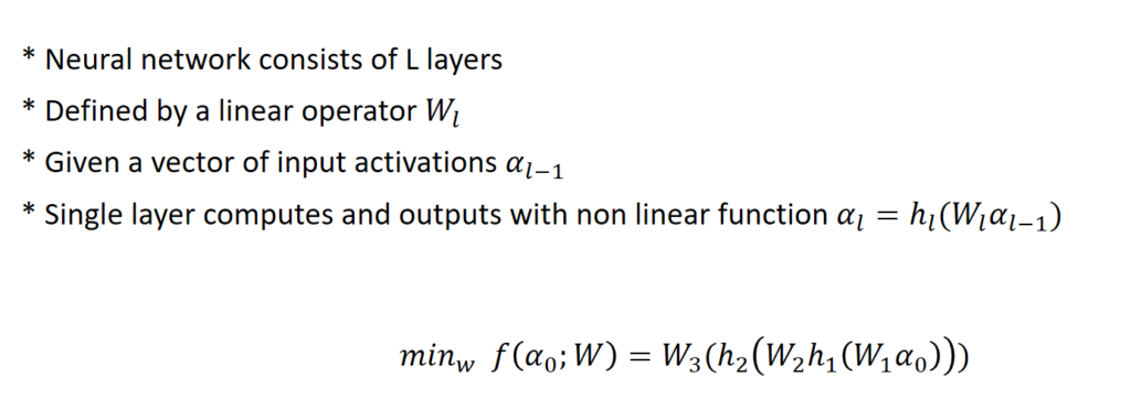 objective function is shown as above.
Model of proposed method
Now, let’s check the model.
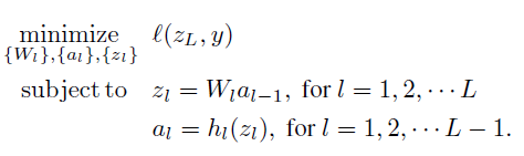
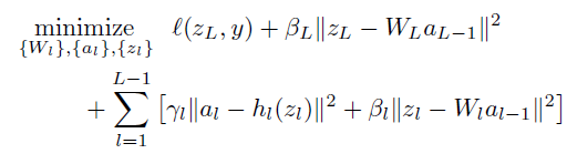
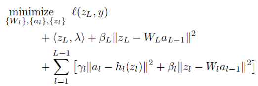
we want to minimize loss function. Two constraint is corresponding to the constraint that I explained above. To make unconstrained problem, they use penalty term .
Proposed method use lagrange multiplier only related with objective term. Thus the model became as below.
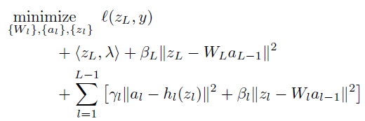
Compare to classical ADMM which use lagrange multiplier to all the constraint, the proposed method only apply to objective term.
This is because as proposed scheme involves more than two coupled variable blocks and non smooth function, it lies outside the scope of known convergence results for ADMM. Thus they cannot apply to all constraints but just objective term and this part is related with bregman iteration in proposed method. The convergence of bregman iteration is well understood in the presence of linear constraints.
Before checking bregman iteration, let’s see the sub-problem which is the property of ADMM scheme in proposed method.
There are several parameters to update in neural network. Weight, input activation and output activation and lagrange multiplier are parameter to be updated.
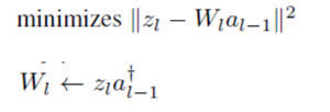
- Weight update (LSE)
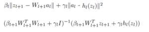
- Activation update (LSE)
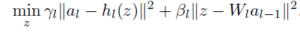
- Output update
Sub problems of updating weight and activation are easy. It can be solved in LSE.
Output update is challenging separable updating in ADMM scheme. However as entries in Z_{l} are decouple, the problem can be decomposes into solving a large number of one-dimensional problems, one for each entry in Z_{l}.
Bregman iteration
Now let’s check the update of largrage multiplier and bregman iteration. We already check that the reason proposed method used bregman iteration.
Bregman distance with a convex function E at the point v is 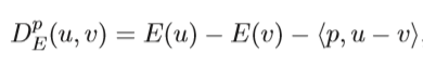
Geometrically we can interpret as below
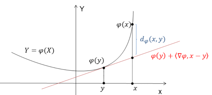
which is the distance between function value and tangent line.
Starting from minimize convex function E and linear constraint H and penalty coefficient lambda, bregman iteration perform as below.

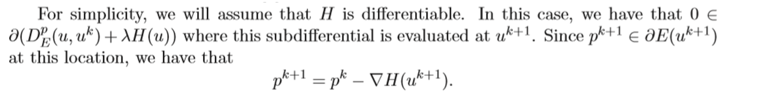
Thus, we checked that how does the subgradient is updated in bregman iteration.
Let’s come back to our problem.
with respect to Z_{l} we can obtain
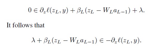
we can check above equation is identical to update equation of subgradient in bregman iteration. Thus, we could interpreted as largragian multiplier as subgradient in bregman iteration.
I think this is the reason the largrangian multiplier is applied to only objective term. To use bregman iteration, they need the largrangian multiplier term related with objective function to update as subgradient in bregman iteration.
Below is the algorithm for proposed method what I mentioned until now.
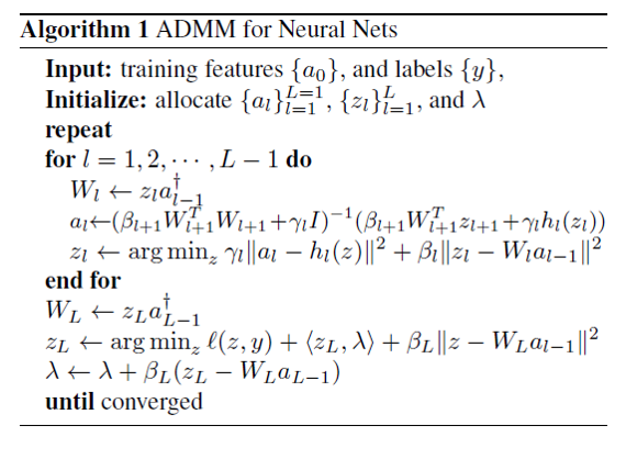
Implementation & Data parallel
- Distributing the algorithm across N worker nodes. (CPU parallel computation)
- Different nodes store activations and outputs corresponding to different subsets of training data.
- To start good initial value for converge, they used proposed method by running several iterations without largrangian multiplier updates at first.
- set large value in penalty coefficients.
- Training data is binary class label
- Loss function is hinge penalty form which is convex function.
Experiment Result
- They compare the proposed method with gradient-based method with GPU computation which is conjugate gradients, SGD and L-BFGS.
SVHN DATA
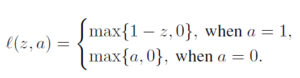
First, they focus on the problem posed by the SVHN dataset. For this dataset, they optimized a net with two hidden layers of 100 and 50 nodes and ReLU activation functions. The data is relative small and easy to train.
Above is the result. First graph shows that time required for proposed method to reach 95% test accuracy vs number of cores. We can check the advantages of scaling of proposed method. Second graph shows test set predictive accuracy as a function of time in seconds for each method. We can not say that proposed method have outperformance to other method.
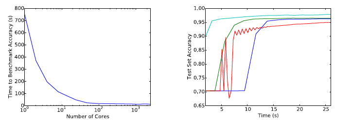
Second, they focus on Higgs dataset which is relative larger and difficult to train. They optimized a simple network with ReLU activation function and a hidden later of 300 nodes.
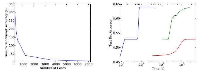
Above is the result. From the first graph, we can still check the scalability of the proposed method. From the second graph, the proposed method ( blue ) have outperformance in this dataset than the methods based on gradient with GPU computation.
Conclusion
- They present a method for training neural networks without using gradient steps.
- Proposed method avoid many difficulties of gradient method.
- Performance of the proposed method scales linearly up to thousands of cores.
- Proposed approach out-perform other methods on problems involving extremely large datasets.