Author: jiamin

Author: Jiamin Wang and Spencer Jenkins

Motivation

Basically, machine learning problem is about function approximation. If we have datasets (x, y), x is the variables and y is the response, and we want to fit some function f, parameterized by some parameter vector θ, f(x,θ), to predict y. In neural network framework, the fitted function is usually nonlinear. We can define the loss function measuring how well function f’s prediction. Finally, some local optimization algorithm can be employed to minimize the loss function. 

minimize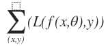

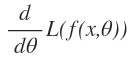
If we want to calculate the minimum of loss function, we need compute the derivative of loss function with respect to the parameter .

But the loss function obtained from neural network model is very large, so that we can’t generally write it down in any closed-form. There is one example provided in the blog:

f(x)=exp(exp(x) + exp(x)^2) + sin(exp(x) + exp(x)^2)

If we compute the derivative using symbolic differentiation,which the ‘flat’ version of this function.  The math expression show:

df/dx=exp(exp(x)+exp(x)^2)(exp(x) +2exp(x)^2) + cos(exp(x) +exp(x)^2)(exp(x)+2exp(x)^2)

It isn’t too hard to explicitly write down this equation. However the actual loss function is even much more complicated, and the derivative will explode.

Automatic differentiation

In a smart way, we can use the automatic differentiation(autodiff), which has two modes forward and reverse. In neural nets framework, reverse mode of autodiff is also called back propagation. Both of these two modes need to calculate f(x) and become slow when the input variable is in high dimension.

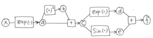
What is autodiff, autodiff is compute the derivative by defining some intermediate variables as shown below:

a=exp(x)

b=a^2

c=a+b

d=exp(c)

e=sin(c)

f=d+e

It is convenient to draw the graph to illustrate the relationship between all the intermediate variables. We can work backwards to calculate the derivative of f with respect to each variable by the chain rule.

            

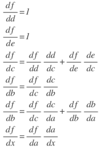
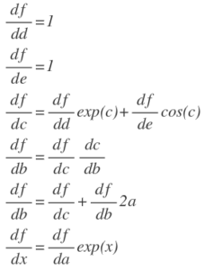
In this way, we can compute the derivative of each variable and make use of the derivatives of the children of that variable.

• The general formulation of forward propagation. Variable are the input and 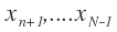are the intermediate variables, is the final value. The functionsare defined as the elementary functions evaluated on the ‘parents’ Pa(i) of variable i. The formulation of forward propagation is

For i=n+1, n+2….N:

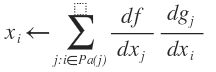
• The general formulation of backward propagation. The derivative of function f with respect to the final value

For i = N-1, N-2,….1:

Advantages of Autodiff

Space complexity: Autodiff has fewer thing to memorize. The rules for transforming the code for a function into code for the gradient are really minimal.

Time complexity: The program for the gradient has exactly the same structure as the function, which implies that we have the same runtime.

Autodiff by the method of Lagrange multipliers

Intermediate variables are the equality constraint in the optimization problem. Blog example can be written in this constraint form:

argmax f

s.t.  a=exp(x)

b=a^2

c=a+b

d=exp(c)

e=sin(c)

f=d+e

The general formulation

• Input variables: 

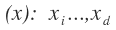
• Intermediate variables: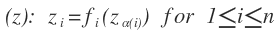, the term is the parents of i.
• Output variable(): we assume the programs have a singled scalar output variable  which represents the quantity we want to maximize.

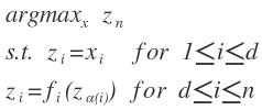
The standard way to solve the constrained optimization is to converts the constrained optimization problem into an unconstrained formula with parameters , called Lagrange multipliers.

The really interesting result in this blog post comes from applying the method of Lagrange multipliers to the constrained optimization form of our problem as shown above. By introducing additional variables (known as Lagrangian multipliers), we can turn our problem into an unconstrained optimization problem which takes the following form:

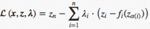
We call the above form the Lagrangian. To optimize our Lagrangian, we take its gradient and set it equal to zero. We then solve for our Lagrange multipliersand our intermediate variables .

The original blog post does a good job of deriving the results of this optimization, so we won’t go into too much detail on the process. The main results, however, are summarized below:

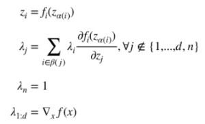
There are a few interesting things to observe from the results of the Lagrangian method. First, we can see that satisfying the constraints on our intermediate variables can be interpreted as the feedforward step in backpropagation. Second, we can see that the result we get for our Lagrangian multipliers is of the same form as what we get during backpropagation. We are summing all λ that directly depend on j, scaling each by the derivative that relates i and j. This is an equivalent operation to determining our δ terms in backpropagation. Lastly, we see that we can solve for our Lagrange multipliers and our intermediate variables by performing back-substitution. We cannot, however, obtain a closed-form solution for our input variables. We can only solve for  and thus obtain the gradient of our original function. To solve for the input variables, we will have to perform something like gradient ascent.

The author goes on to briefly describe how cyclic constraints could also be handled by this approach. The feedforward procedure becomes more difficult and a linear solver is required to determine the Lagrangian multipliers, but the procedure essentially stays the same.

The main benefit of thinking about backpropagation in the Lagrangian sense is the ability to apply constrained optimization algorithms to our problem. The author doesn’t go into much detail on use cases and benefits for this approach, but it isn’t hard to imagine that considering other algorithms might prove useful given certain problems. The connection between backpropagation and the method of Lagrange multipliers is more than just a curiosity.

As a final note, we found the following paper helpful in understanding the ideas presented in the blog post: A Theoretical Framework from Back-Propagation (LeCun, 1988). It presents the same idea as the blog post, organized in a very similar manner. The notation in this paper is more closely related to how backpropagation is typically formulated (the blog post deals with a slightly more general form), so the connection between backpropagation and the method of Lagrange multipliers might become more clear after reading this resource.