This post presents a summary of the background and class discussion on the Adam (adaptive moment estimation) algorithm. The primary source for this discussion was the original Adam paper. Adam is quite possibly the most popular optimization algorithm being used today in machine learning, particularly in deep learning.
Background (Ryan Kingery)
Adam can be thought of as a generalization of stochastic gradient descent (SGD). It essentially combines three popular additions to SGD into one algorithm: AdaGrad, Nesterov momentum, and RMSProp.
Adam = AdaGrad + momentum + RMSProp
Recall from a previous post that AdaGrad modifies SGD by allowing for variable learning rates that can hopefully take advantage of the curvature of the objective function to allow for faster convergence. With Adam we extend this idea by using moving averages of the gradient moment estimates to smooth the stochastic descent trajectory. The idea is that smoothing this trajectory should speed up convergence by making Adam converge more like batch gradient descent, but without the need of using the entire dataset.
To discuss momentum and RMSProp we must recall the definition of an exponentially weighted moving average (EWMA), also called exponential smoothing or infinite impulse response filtering. Suppose we have a random sample 


The hyperparameter 


The EWMA is useful when we’re given noisy data and would like to filter out some of the noise to allow for better estimation of the underlying process. We thus in practice tend to favor higher values of 
It turns out that the EWMA tends to produce bias estimates for the early values

One might naturally ask whether this bias correction term is something to worry about in practice, and the answer, of course, is it depends. The time it takes for the bias to go away goes roughly like 


In the context of machine learning though, it doesn’t really make much of a difference when you’re training for many thousands of iterations anyway. To see why, suppose you have a modest dataset of 10,000 observations. If you train this using a mini-batch size of 32, that gives about 312 iterations per epoch. Training for only 10 epochs then already puts you over 3000 iterations. Thus, unless you’re in a scenario where you can train your data very quickly (e.g. transfer learning), the bias correction probably won’t be important to you. It is thus not uncommon in practice to ignore bias correction when implementing EWMA in machine learning algorithms.
Now, the Adam algorithm uses EWMA to estimate the first and second order moment estimates of the objective function gradient 
Recall that the 


We can see then that the first moment is just the expectation 
For a random vector 

and the second moment component-wise by

Back to Adam again, denote the gradient 


In practice, it’s common to take 


Note that the bias corrected terms are included in the update! This is because the authors of the paper did so, not because it’s usually done in practice, especially for the momentum term 

The ratio 

We thus now have a “smoother” version of AdaGrad that allows for robustness in the presence of the noise inherent in SGD. Whether the algorithm holds in practice is a question that has repeatedly been validated in numerous deep learning applications. Whether this actually helps in theory leads to a discussion of the algorithm’s convergence “guarantees”.
Convergence (Colin Shea-Blymyer)
The proof of convergence for this algorithm is very long, and I fear that we won’t gain much from going through it step-by-step. Instead, we’ll turn our attention to an analysis of the regret bounds for this algorithm.
To begin, we’ll look at what regret means in this instance. Formally, regret is defined as
![R(T) = \sum\limits_{t=1}^T[f_t(\theta_t)-f_t(\theta^*)].](https://s0.wp.com/latex.php?latex=R%28T%29+%3D+%5Csum%5Climits_%7Bt%3D1%7D%5ET%5Bf_t%28%5Ctheta_t%29-f_t%28%5Ctheta%5E%2A%29%5D.&bg=ffffff&fg=000&s=0&c=20201002)
In English, that represents the sum how far every step of our optimization has been from the optimal point. A high regret means our optimization has not been very efficient.
Next we’ll define 


![g_{1:t,i} = [g_{1,i}, g_{2,i}, ..., g_{t,i}].](https://s0.wp.com/latex.php?latex=g_%7B1%3At%2Ci%7D+%3D+%5Bg_%7B1%2Ci%7D%2C+g_%7B2%2Ci%7D%2C+...%2C+g_%7Bt%2Ci%7D%5D.&bg=ffffff&fg=000&s=0&c=20201002)
That is, a vector that contains the 
![\frac{\beta_1^2}{\sqrt[]{\beta_2}}](https://s0.wp.com/latex.php?latex=%5Cfrac%7B%5Cbeta_1%5E2%7D%7B%5Csqrt%5B%5D%7B%5Cbeta_2%7D%7D&bg=ffffff&fg=000&s=0&c=20201002)


The next step is to make some assumptions. First, assume the gradients of our function 


Finally, we define some ranges for our parameters: 


Now we are armed to tackle the guarantee given for all 

To make analysis of this easier, we’ll refer to specific terms in this inequality as such:

Allowing each summation, and fraction without summation be a separate term.
Term 


We’ll start with the numerator: the learning rate, the decay of the first moment, and the maximum Chebyshev magnitude of our gradients – all aspects that allow for a larger regret when endowed with large values. In the denominator we have subtractive terms, so to maximize regret, the decay of the second and first moments, and (something like) the ratio between them should all be small. 
This, for me, is the hardest part to gain an intuition of. Finally, we find ourselves at 
Looking back through this, we can start to see how certain terms effect how large the regret of the algorithm can be: the 


Finally, by accepting that

we find that 


 is the ith entry of the Riemannian metric tensor
  (a positive definite matrix of size n x n)
 , the update rule using gradient descent is

 is the inverse of the Fisher information matrix. Does this remind you of something you have seen before? Yes, this update rule is identical to that of the Newton method with the only difference being that
  , also natural gradient does not assume that
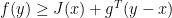 for all y.
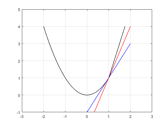

 is subgradient of
  .
. ):
):
 for all
  , i.e.,
  .
. of the algorithm with the optimum value
  is bounded, i.e.,
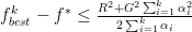
 , we find different values for the bound. Two step sizes that we went through their detail in the class were:
 : which is a positive constant. In this case, we will have
 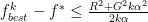 . As
. As  .
. ,
, 

 iterations. To compare it with the gradient descent method, we have to note that if
  , then it only needs 10 iterations in gradient descent. However, this gradient descent convergence rate is for strongly convex case only.
 for the true (sub)gradient
  at every point
  , which satisfies
 denotes the expected value of
 is the step size.
 , the expected error in function value is given by
 is the true optimal value for
  need only be convex with a subgradient. Now, using a constant step size
  , robust SGD can be proven to converge to some neighborhood of the true minima
  at a rate of
  . It follows, that for a general function, it is good practice to begin SGD with a constant step size, then diminish the step size whenever the algorithm seems to have stalled in its progress.
 .
. for which
 ,
, such that
 .
. ,
, is considered a constant, and
  is the value of
  ,
, .
. ,
, .
. and
and  , and the secant condition is
 .
. ,
, and
and  are the shorthand used to describe these difference vectors in the slides. Based on the existence of these outer products, it appears as if an
  cost is unavoidable, when all the literature says the memory and running time costs are
  .
. . We then have products of length-
 ,
, .
.