Natural Gradient Explained

In machine learning (supervised learning), we train a model by minimizing a loss function that outputs the difference between our prediction given a data point and the true label of that data point. Learning is cast as an optimization problem and often we use gradient descent or its variants to seek solution to this problem.

In the previous post we learnt about Gradient Descent, Newton’s method and LBFGS optimization techniques. In this post we will cover natural gradient, its formulation, usage and applications in machine learning.

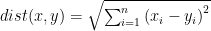
To understand natural gradient, we need to revise our understanding of distance. We define the distance between two points $x, y \in \mathbb{R}^n$ in Euclidean space as

$dist(x, y) = \sqrt{\sum_{i = 1}^{n} {(x_i - y_i)}^2}$

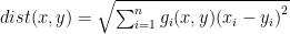
This distance measure is not appropriate if our function of interest lies in a different geometric space other than the Euclidean space. Natural gradient employs this property by giving the distance between two points $x, y \in \mathbb{R}^n$ that lie in a Riemannian space as

$dist(x, y) = \sqrt{\sum_{i = 1}^{n} g_i(x,y){(x_i - y_i)}^2}$

where $g_i$ is the ith entry of the Riemannian metric tensor $G(x,y)$ (a positive definite matrix of size n x n)

The Riemannian metric tensor that is used in natural gradient formulation is the Fisher information matrix

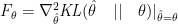
$F_{\theta} = \nabla_{\hat\theta}^2 \textit{KL}(\hat\theta \quad || \quad \theta)|_{\hat\theta = \theta}$

Fisher information matrix is the second derivative of the KL-divergence. For anyone familiar with statistics, KL-divergence is a measure to determine how close a probability distribution is from another probability distribution.

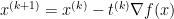
Putting it all together, recall for the optimization problem $\min_{x \in \mathbb{R}} f(x)$ , the update rule using gradient descent is

$x^{(k+1)} = x^{(k)} - t^{(k)} \nabla f(x)$

For natural gradient, we update the parameters of our function using

$x^{(k+1)} = x^{(k)} - t^{(k)} F^{-1} \nabla f(x)$

where $F^{-1}$ is the inverse of the Fisher information matrix. Does this remind you of something you have seen before? Yes, this update rule is identical to that of the Newton method with the only difference being that $F^{-1}$ in Newton is the inverse of the Hessian matrix of $f(x)$ , also natural gradient does not assume that $f(x)$ is approximately locally-quadratic.

Now that we have learnt what natural gradient is and how it is formulated, we ask the question why isn’t this method popular in machine learning and what problems are they good for solving? In practice, natural gradient method is applied to a variety of problems, variational inference, deep neural networks, reinforcement learning and in some cases it performs better than conventional methods e.g. stochastic gradient descent. The main limitation of natural gradient method is that we need to know the Riemannian structure of the parameter space of our function in order to derive its update rule and deriving the algorithm for that can be complex. Also, applying the algorithm can be computationally intensive.

In this post, we have learnt about natural gradient and that it performs better than conventional optimization methods when applied to some problems. I will strongly encourage anyone seeking a more in depth coverage of natural gradient adaptation to check out this paper, or alternatively, this paper to get a concise explanation with mathematical derivations.

Leave a Reply Cancel reply