(Nesterov) Accelerated Gradient Descent

We define standard gradient descent as:
w^{k+1} = w^k - \alpha \Delta f(w^k)

Momentum adds a relatively subtle change to gradient descent by replace f with z. Where
z^{k+1} = \beta z^k + \Delta f(w^k)
w^{k+1} = w^k - \alpha z^{k+1}

As such, alpha retains the role of representing the step size. However, we introduce a new constant, beta. Beta adds a decaying effect on momentum, and must be between 0 and 1, noninclusive. We briefly demonstrate the edge cases of beta below:
\beta = 0:    w^{k+1} = w^k + \alpha \big ( 0 \times z^k + \Delta f(w^k) \big )    \rightarrow    w^{k+1} = w^k +\alpha \Delta f(w^k)
\beta = 1: w^{k+1} = w^k - \alpha \big (    \Delta f(w^k) + \Delta f(w^{k-1}) + \Delta f(w^{k-2}) + \dots    \big )

We now introduce a change of basis which will be convenient for later. Consider a matrix form of gradient descent:
w^{k+1} = w^k - \alpha (Aw^k - b) \text{ where } \Delta f(w) = Aw^k-b 

Which has optimal solution
w^{\star} = A^{-1}b 
we consider the eigenvectors of A which is a natural space of viewing A where all dimensions act independently.

Given:
$latex A = Q \text{ diag }(\lambda_1 \dots \lambda_n)Q^T $
x^k = Q^T (w^k - w^{\star})    \leftarrow \text{new basis}

We may derive this by:
w^{k+1} = w^k - \alpha (Aw^k - b) 
w^{k+1} -w^{\star} = w^k - w^{\star} - \alpha (Aw^k - b) 
Q^T\big(w^{k+1} -w^{\star}\big) = Q^T\big(w^k - w^{\star}\big) - \alpha Q^T \big(Aw^k - b\big ) 
x^{k+1} = x^k - \alpha Q^T \big(Aw^k - b\big ) 

w^{\star} = A^{-1}b    \implies    Aw^{\star} = b
x^{k+1} = x^k - \alpha Q^T \big(Aw^k - Aw^\star \big ) 
x^{k+1} = x^k - \alpha Q^T A \big (w^k - w^\star \big ) 
x^{k+1} = x^k - \alpha Q^T Q \text{diag}\big(\lambda\big)Q^T \big (w^k - w^\star \big ) 
x^{k+1} = x^k - \alpha \text{diag}\big(\lambda\big)Q^T \big (w^k - w^\star \big ) 
x^{k+1} = x^k - \alpha \text{diag}\big(\lambda\big) x^k 
x_i^{k+1} = x_i^k - \alpha \lambda_i x_i^k    = (1- \alpha \lambda_i )x_i^k
$latex = \sum_i^n x_i^0(1-\alpha \lambda_i)^k q_i $

Thus, we now can view gradient descent in basis of the eigenvectors of A. We consider the contributions of error as
$latex f(w^k)-f(w^\star) = \sum (1 – \alpha \lambda_i)^{2k} \lambda_i [x_i^0]^2 $
For convergence, we note that
$latex 1 – \alpha \lambda_i $
must be strictly less than 1.


Note: To be continued…

Visualizing the Loss Landscape of Neural Nets

Introduction

The performance of Neural Networks could be affected by the landscape of loss function, which is decided by a wide range of factors including network architecture, the choice of optimizer, variable initialization, etc. Studying and visualizing the effect of these factors on the underlying loss landscape is challenging because they often lie in high-dimensional spaces and are hard to be captured geometrically, while human perceivable visualizations are only low-dimensional 1D (line) or 2D (surface) plots. The paper we read is therefore motivated to close this dimensionality gap and proposes visualization method that can enable meaningful side-by-side comparisons.

Basics

Given input data (feature vectors {xi} and accompanying labels {yi}), neural network losses are high-dimensional non-convex functions computed with the parameter set \theta. The paper first reviews two conventional method to visualize the loss landscape:

1-Dimensional Linear Interpolation

Choose two sets of parameters \theta and \theta', move by certain scale from one point to another along the line connecting these two points and plot the values of the loss function. The points along the line can be computed with a weight parameter \alpha by \theta(\alpha) = (1-\alpha)\theta + \alpha \theta'.

2D Contour Plots

Choose a center point \theta^*, either choose one direction \delta to move along and plot a function of the form f(\alpha)=L(\theta^*+\alpha\delta), or choose two directions, \delta and \eta, plot a 2D surface of the form f(\alpha, \beta) = L(\theta^* + \alpha\delta + \beta\eta). The 2D plotting is more computationally costly, so the method often produces low-resolution plots of small regions.

Filter Normalization

Scale Invariance

When random directions are used in visualization, the plots are sensitive to the scale of model weights. “A neural network with large weights may appear to have a smooth and slowly varying loss function”. However, neural networks are scale invariant, especially when batch normalization is applied to rescale the output of each layer.

Filter Normalization

In order to remove the scaling effect and enable meaningful comparisons between plots, the paper proposes to use filter-wise normalized directions. Given a random Gaussian direction d with dimensions compatible with parameter with \theta, each filter in d is normalized to have the same norm of the corresponding filter in \theta

where d_{i,j} represents the j^{th} filter (not the jth weight) of the i^{th} layer of d.

The Sharp vs. Flat Delemma

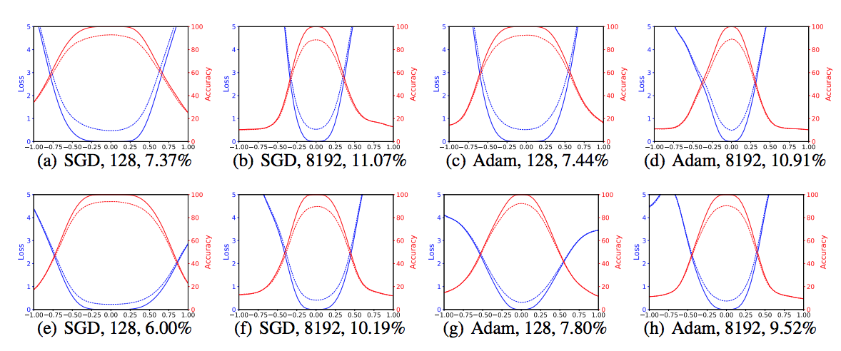
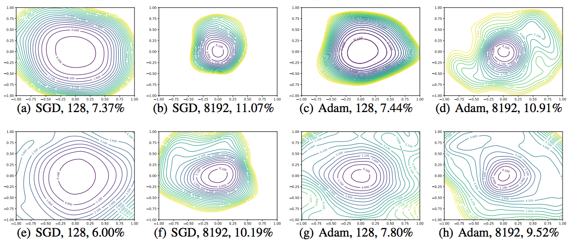
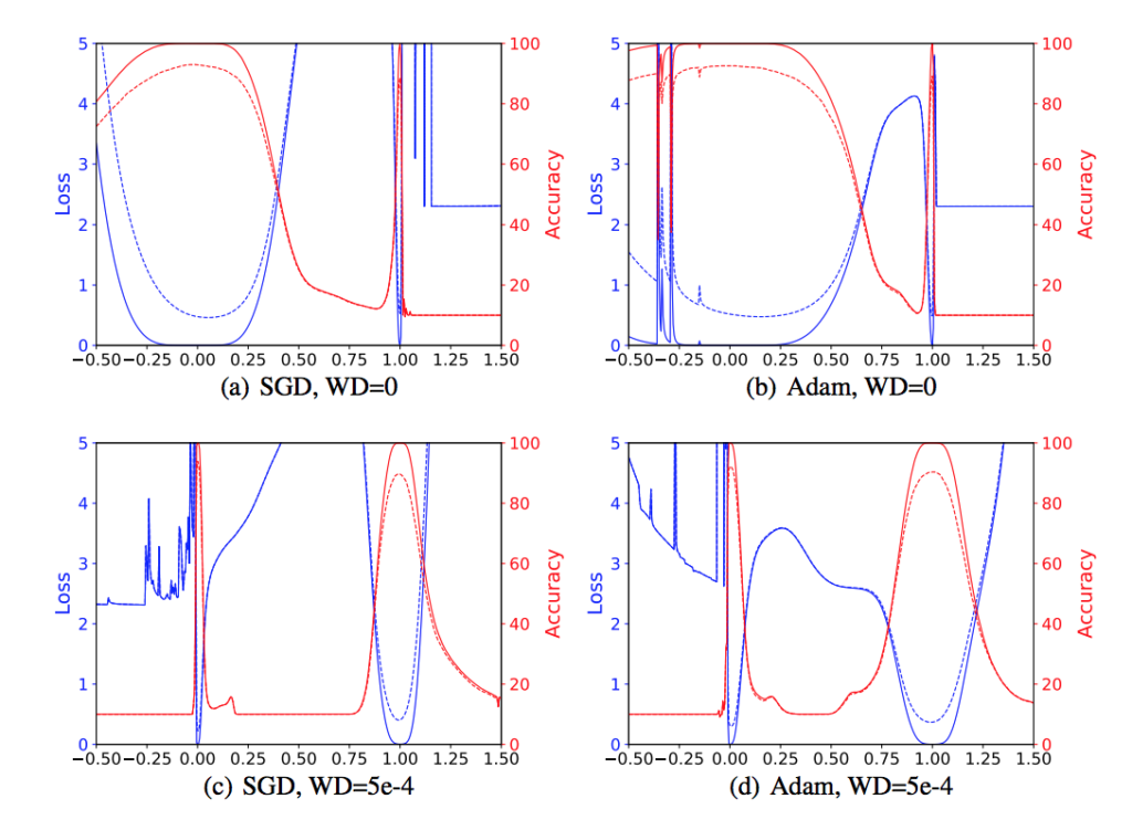
The authors then applied filter normalized directions to study whether sharp minimizers generalize better than flat minimizers. It is widely believed that small-batch SGD usually produces “flat” minimizers while large batch sizes produce “sharp” minima with poor generalization”, so they train a CIFAR-10 classifier using a 9-layer VGG network, running SGD with small batches and large batches produces solution \theta^s and \theta^l respectively. Then they plot 1D interpolation plots between \theta^s and \theta^l. However, as shown in the figure below, with these plots, there is no apparent correlation between sharpness and generalization because it can easily flipped by turning on a small weight decay.

The flipping is because adding weight decay reduces the scale of weights, small weights are more sensitive to perturbation and therefore produce sharper looking minimizers.

Then they apply filter normalized directions to make 1D and 2D plots. These plots remove the effect of the scale of weights, and from the results, we can make meaningful side-by-side comparisons and conclude that large batches do produce sharper minima with higher test error.

Skip Connections and Dropout

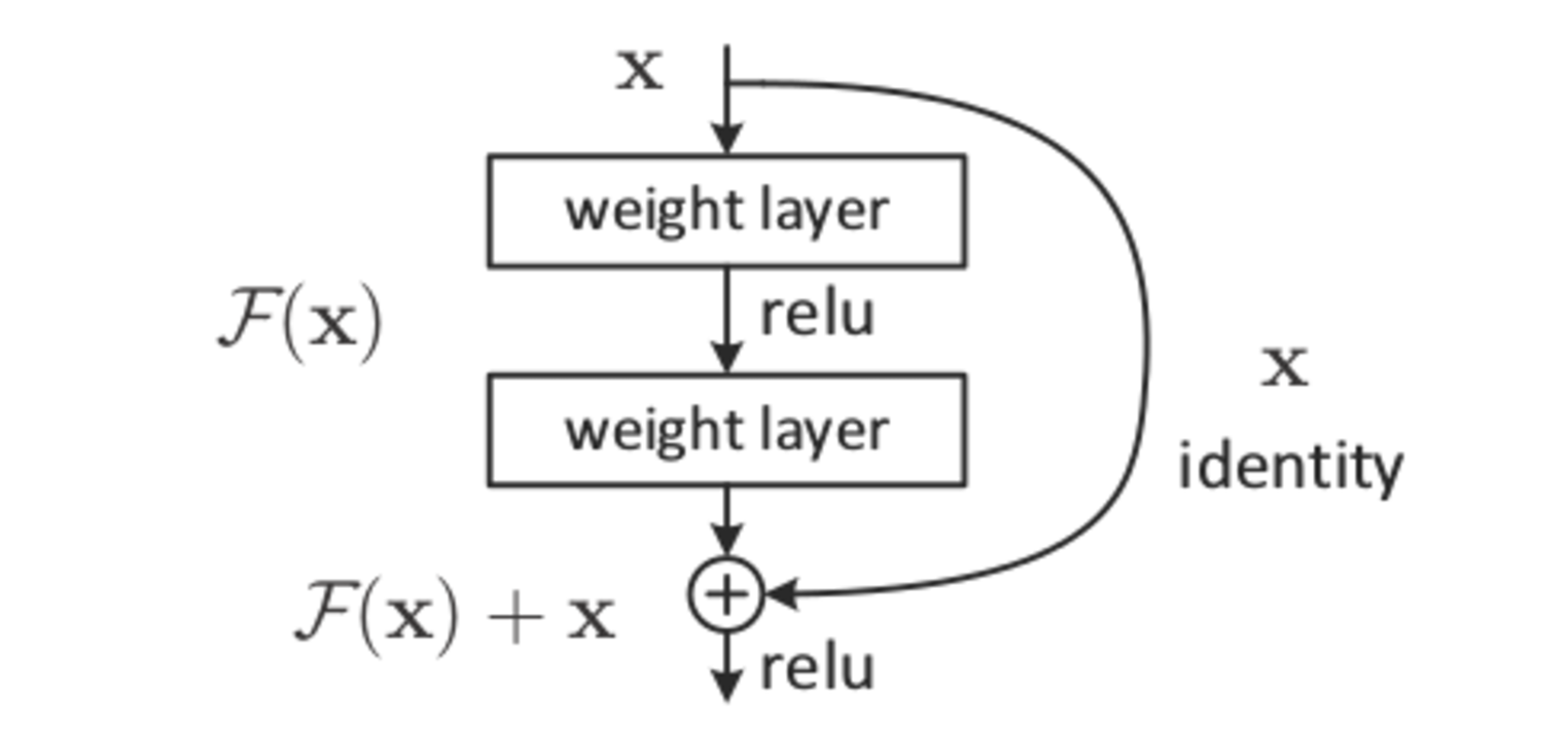
This paper mentions skip connections, which is a method commonly used in very deep networks in order to preserve the values of the input batches through the decay caused by the vanishing gradient problem. In essence, the output of some layers are directly inputted into layer much further down in the network, networks which utilize this are called Residual networks and are the basis for the current SOTA on images. This method is different from dropout, which gives a probability for certain neurons in a network to just output zero no matter their inputs. Both of these methods supposedly help a network in generalization, but there are no real mathematical justifcations for either – just experiments which show networks performing better when using these techniques.

Skip Connection
Skip Connections

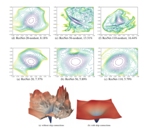
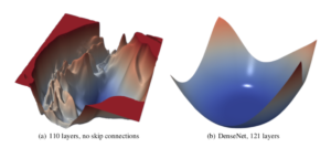
This paper attempts to show that the practical affects of adding these methods are actually realted to the loss surface of the network. They increase the overall convexity of the surface and have a smoothing effect, which means that the random initalization of the weights has a higher probability to be in an “escapeable” region of the loss surface that will converge to a local minima.

“For the more shallow networks (ResNet-20 and ResNet-20-noshort), the effect of skip connections is fairly unnoticeable. However residual connections prevent the explosion of non-convexity that occurs when networks get deep.”

Wide vs. Thin Models

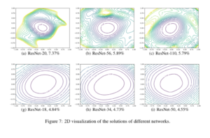
“Increased network width resulted in flat minima and wide regions of apparent convexity”

In this figure, Resnet 18/34/50 contain more convolutional filters per layer than Resnet 20/56/110 and are also shallower, which means less inherent non-convexity according to this paper

Depth causes non-convexity

As network depth increases, this paper notes that “VGG-like” (or very deep networks without residual connections) transition from nearly convex to chaotic loss surfaces. This chaos also has a effect on the sharpness of the minima of the loss surface, where these chaotic surfaces have much sharper minima and the counters near these are perturbed as well so that optimization is doubly difficult. However, by simply adding residual (skip) connections in the very deep network, this effect is easily reversed.

Optimization Paths

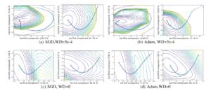
In high dimensional space, two randomly chosen vectors have a very high chance to be nearly orthogonal, meaning that this is very little variance between them. Therefore this paper uses PCA in order to carefully choose two vectors to show descent on, which is especially useful if the descent path is in very low dimensions. The authors of this paper make the claim that 40-90% of variation in the descent path lies in only two dimensions, which means using those two dimensions to produce the optimization path will result in nicely visually descent towards a convex attractor.

Conclusion

Quite a bit of discussion towards the end of our presentation was around the actual helpfulness of visualization methods, and whether using other statistical measures would provide for more information to anyone trying to learn about a network or problem.

Our hesitant conclusion was that visualization itself is a sort of statistical measure which can be used to represent a bunch of smaller measures like convexity, average etc. but for troubleshooting a network it probably isn’t very useful. These techniques are more readily used to quickly convey these overall statistical measures during a presentation or to show quick comparisons of networks to possibly show progression in design. At the very least, these visualizations provide some sort of insight into dropout and residual connections which are currently used in the industry because they work without any real mathematical justification.

Linear Convergence of the Primal-Dual Gradient Method for Convex-Concave Saddle Point Problems without Strong Convexity

Introduction

The convex-concave saddle point problem has the following format:

For many machine learning applications, their objective functions can be written in the convex-concave format. The example applications include reinforcement learning, empirical risk minimization and robust optimization etc.

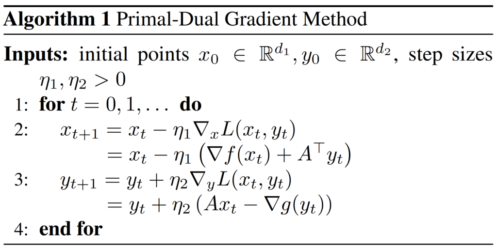
We can use the following primal-dual gradient method to optimize the L(x,y).

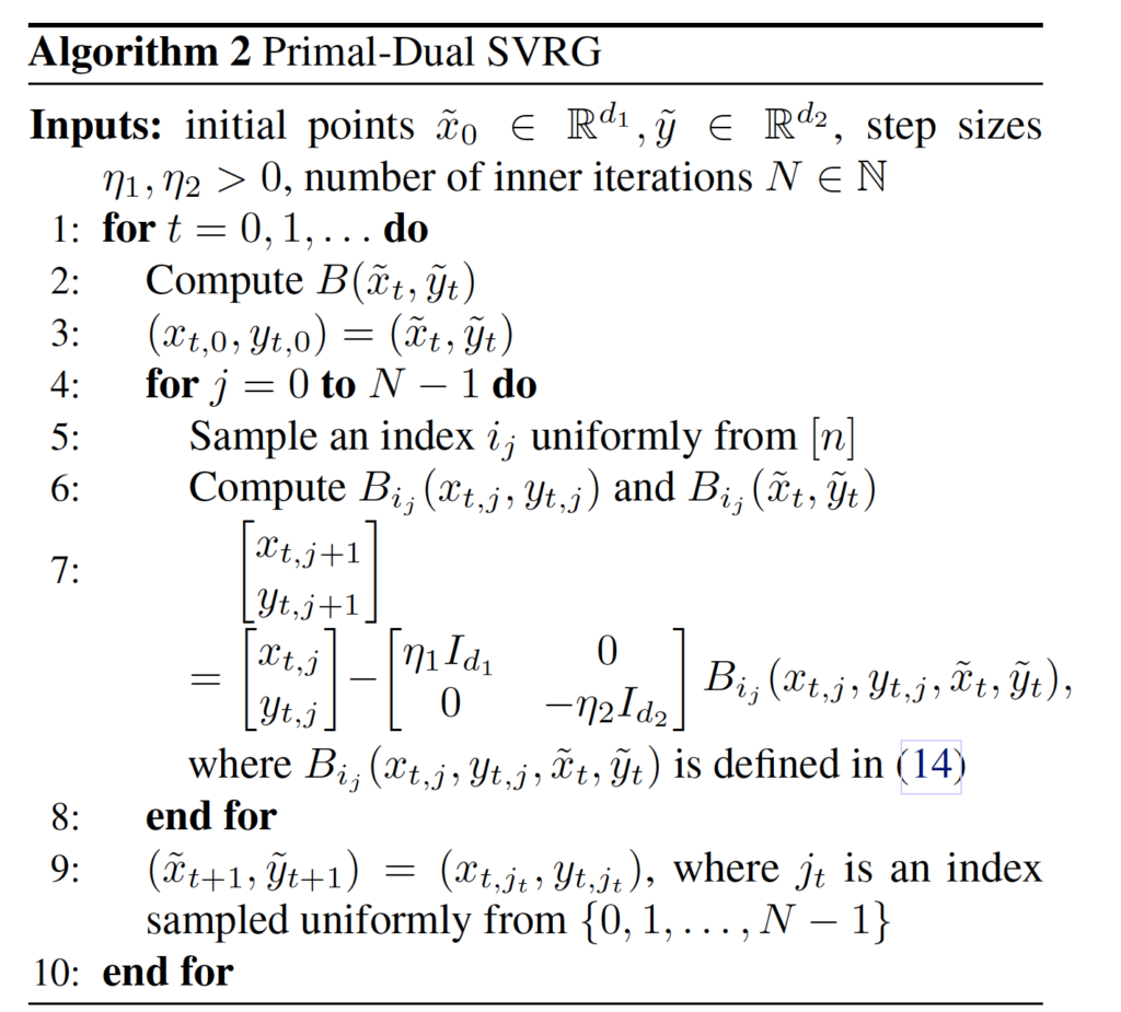
In this paper, the authors develop a new method to prove that the primal-dual gradient method has linear convergence rate, when the f  and g  are smooth, f  is convex, g is strongly convex and the coupling matrix A has full column rank(Section 3). They also extend the primal-dual method to the stochastic situation and propose the primal-dual stochastic variance reduced gradient(SVRG) method. They use the new method to prove that the primal-dual SVRG method also has linear converge rate(Section 4).

Preliminaries

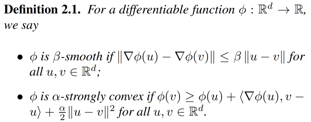
Before we prove the convergence of the primal-dual method, we need some preliminaries. First, we need the definitions of smoothness and strong convexity.

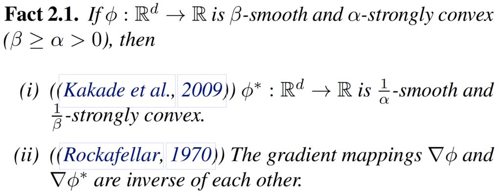
We also need the definition and some properties of  the conjugate function.

Based on the definition of conjugate function, we can get the corresponding primal problem of the L(x,y).

Finally, we need the of gradient descent on the strongly convex function.

Linear Convergence of the Primal-Dual Gradient Method

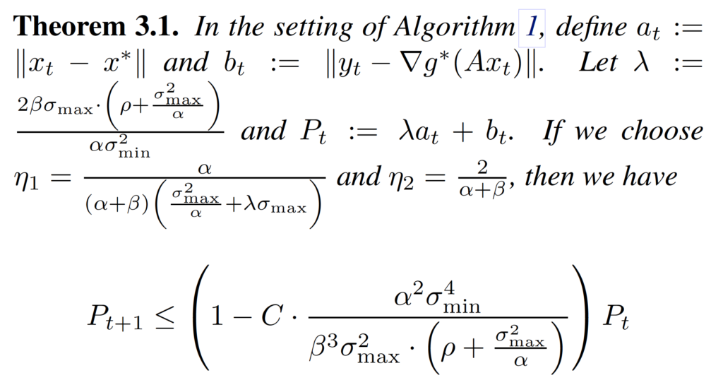
With these preliminaries, we can start to prove the convergence of primal-dual gradient method. The Theorem 3.1 establishes the linear convergence guarantee for it.

This theorem says that if we construct a Lyapunov function P_t = \gamma a_t + b_t, we can prove that the function satisfies the condition that P_{t+1} \le (1-c)P_t, which implies the linear convergence rate.

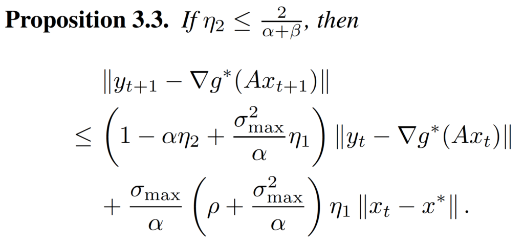
We can divide the proof of this theorem to three steps. First, we bound the decrease of a_t. That is, we want to prove that a_{t+1} \le c_1 a_{t} + c_2 b_t. Second, we bound the decrease of b_t. Finally, we prove the inequality.

Proposition 3.1 and Proposition 3.2 give the bound of decrease of a_t.

The proof technique of the first step is to first find the relationship between a_t and ||\tilde{x}_{t+1} - x^*||, and the relationship between x_{t+1} and \tilde{x}_{t+1}. And then use the triangle inequality to find the relationship among a_{t+1}, a_t and b_t. The authors call the \tilde{x}_{t+1} ghost variable in this paper, which is actually the $x$ obtained by updating the x_t with the true gradient, i.e., \nabla P(x).

Proposition 3.3 and Proposition 3.4 give the bound of decrease of b_t. We can use the convex function’s property to prove them.

After we have these propositions, we can put them together, and with some routine calculations, we can prove the inequality in Theorem 3.1.

Extension to the Primal-Dual Stochastic Variance Reduced Gradient Method

In this section, the authors propose the primal-dual SVRG, and prove its convergence using the same proof method in the third section. The primal-dual SVRG is in Algorithm 2.

The framework of primal-dual SVRG is the same as the vanilla SVRG. The main difference is only that the primal-dual SVRG updates the parameters x and y together. In Theorem 4.1, they prove that the primal-dual SVRG also has the linear convergence rate.

Preliminary Empirical Evaluation

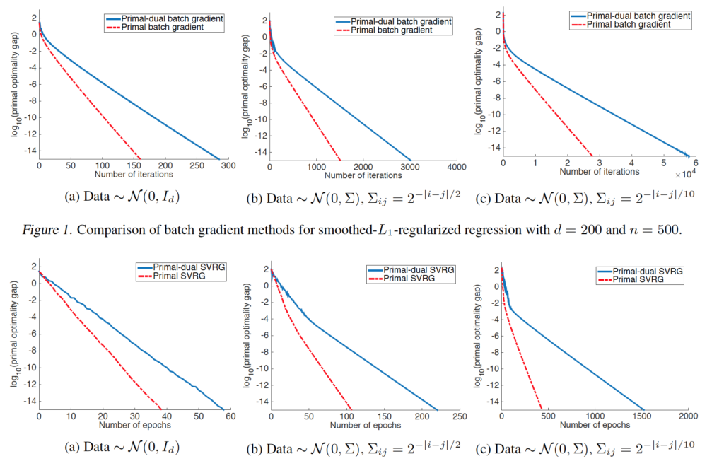
They do experiments on synthetic dataset to prove the convergence of primal-dual gradient method. The results are as below.


On the Global Linear Convergence of Frank-Wolfe Optimization Variants

1.Introduction 

The Frank-Wolfe (FW) optimization algorithm has lately regained popularity thanks in particular to its ability to nicely handle the structured constraints appearing in machine learning applications.

In this section, consider the general constrained convex problem of the form:

\underset { x\in M }{ min } f(x),\quad M=conv(A),\quad with\quad only\quad access\quad to:\quad { LMO }_{ A }(r)\in \underset { x\in A }{ arg min } <r,x>

Where A\subseteq { R }^{ d } is a finite set of vector that we call atoms. Assume that the function f is \mu -strongly convex with L-Lipschitz continuous gradient over M.

2. Original Frank-Wolfe algorithm

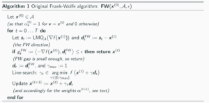
The Frank-Wolfe (FW) optimization algorithm, also known as conditional gradient, is particularly suited for the setup. It works as follows:

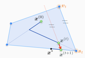
At a current iterate x^(t), the algorithm finds a feasible search atom st to move towards by minimizing the linearization of the objective function f over M – this is where the linear minimization oracle LMOa is used.

The next iterate x^(t+1) is then obtained by doing a line-search on f between x^(t) and st.

3. Variants of Frank-Wolfe algorithm

3.1 Away-Frank-Wolfe Algorithm

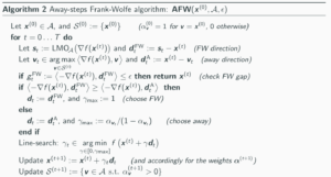
However, there is zig-zagging phenomenon. In order to address this phenomenon, away-Frank-Wolfe algorithm is proposed. Add the possibility to  move away from an active atom in { S }^{ (t) }.

3.2 Pairwise Frank-Wolfe Algorithm

pairwise Frank-Wolfe algorithm is also called MDM algorithm. At first, it proposed to address the polytope distance problem. It hopes to move weight mass between two atoms in each step. According to the algorithm 3, we can know that is almost algorithm 2, except { d }_{ t }={ { d }_{ t } }^{ PFW }:={ s }_{ t }-{ v }_{ t }\quad and\quad { \gamma }_{ max }:={ \alpha }_{ { v }_{ t } }.

4. Global Linear Convergence Analysis

In this paper, section 2 is talking about global linear convergence analysis. We can see that at first, it introduce the proof elements and convergence proof. And lately, section 2.2 is talking convergence results.

4.1 proof of convergence

4.1.1

As f has the L-Lipschitz gradient, we can get

f({ x }^{ (t+1) })\le f({ x }^{ (t) })+\gamma <\nabla f({ x }^{ (t) },{ d }_{ t })>+\frac { { \gamma }^{ 2 } }{ 2 } L{ ||{ d }_{ t }|| }^{ 2 }\quad \quad \forall \gamma \in [0,{ \gamma }_{ max }] (1)

Choose \gamma to minimize RHS:

{ h }_{ t }-{ h }_{ t+1 }\ge \frac { { <{ r }_{ t },{ d }_{ t }> }^{ 2 } }{ 2L{ ||{ d }_{ t }|| }^{ 2 } } =\frac { 1 }{ 2L } { <{ r }_{ t },{ \hat { d } }_{ t }> }^{ 2 } ,when { \gamma }_{ max } is big enough.

4.1.2

By \mu-strong convexity of f, we can get (with { e }_{ t }:={ x }^{ * }-{ x }^{ (t) }):

f({ x }^{ (t) }+\gamma { e }_{ t })\ge f({ x }^{ (t) })+\gamma <\nabla f({ x }^{ (t) },{ e }_{ t })>+\frac { { \gamma }^{ 2 } }{ 2 } \mu { ||{ e }_{ t }|| }^{ 2 }\quad \forall \gamma \in [0,1]

Use \gamma=1 on LHS get:

{ h }_{ t }\le \frac { { { <r }_{ t },{ \hat { e } }_{ t }> }^{ 2 } }{ 2\mu }

4.1.3

combining 4.1.1 and 4.1.2, we can get

{ h }_{ t }-{ h }_{ t+1 }\ge \frac { \mu }{ L } \frac { { { <r }_{ t },{ \hat { d } }_{ t }> }^{ 2 } }{ L{ <{ r }_{ t },{ \hat { e } }_{ t }> }^{ 2 } } { h }_{ t }\ge \frac { \mu }{ L } { <{ \hat { r } }_{ t },{ \hat { d } }_{ t }> }^{ 2 }{ h }_{ t }

Thus, lower bounds * to get linear convergence rate.

5. Conclusion

This paper reviews variant of FW algorithm and shows for the first time global linear convergence for all variants of FW algorithm. It introduces of the notion of the condition number of the constraint set.

6. Reference

1.  Simon Lacoste- Julien & Martin Jaggi: On the global linear convergence of Frank-Wolfe optimization variants.

2. Simon Lacoste- Julien & Martin Jaggi: http://www.m8j.net/math/poster-NIPS2015-AFW.pdf

3. R. Denhardt-Eriksson & F. Statti: http://transp-or.epfl.ch/zinal/2018/slides/FWvariants.pdf


Entropy-SGD: Biasing GD Into Wide Valleys

This is a friendly summary and critical review of the paper “Entropy-SGD: Biasing GD Into Wide Valleys” by Chaudhari et al. (2017) [1].

The post is designed to incrementally deepen the analysis and your understanding of the paper (i.e. you can read the first parts and you will have a birds eye view of what the paper is about).

However, by reading this post in its entirety you will, hopefully, understand the following:

  1. The core problem that motivated this paper.
  2. The historical background and research upon which this paper is based. I highly encourage you to read the papers that I cite. They formulate the foundation of understanding this paper and other methodologically similar papers.
  3. Summarize the important points of the methodology and the algorithm that is utilized.
  4. Important caveats that are not adequately stressed in the paper, especially with respect to the algorithm.
  5. Omissions that should have been included in the paper
  6. Assumptions, especially the one’s that are referenced.
  7. Theoretical properties of the paper and methods of proof.
  8. Resources for the mathematical notation, which is heavily influenced by statistical physics.

Introduction

The authors derive a different Stochastic Gradient Descent (henceforth SGD), which they label as “Entropy – SGD”. The change lies in a modification of the Loss Function of the optimization algorithm. Specifically, they render the the Loss Function “smoother”.

Motivation

Why do they make the Loss Function “smoother”? So that  we have “flat minima” (or “wide valleys” as the authors write, the two terms can be used interchangeably).

Let’s see what this cryptic notion of “flat minima” is all about. Watch carefully the following Figures 1 and 2.

Figure 1
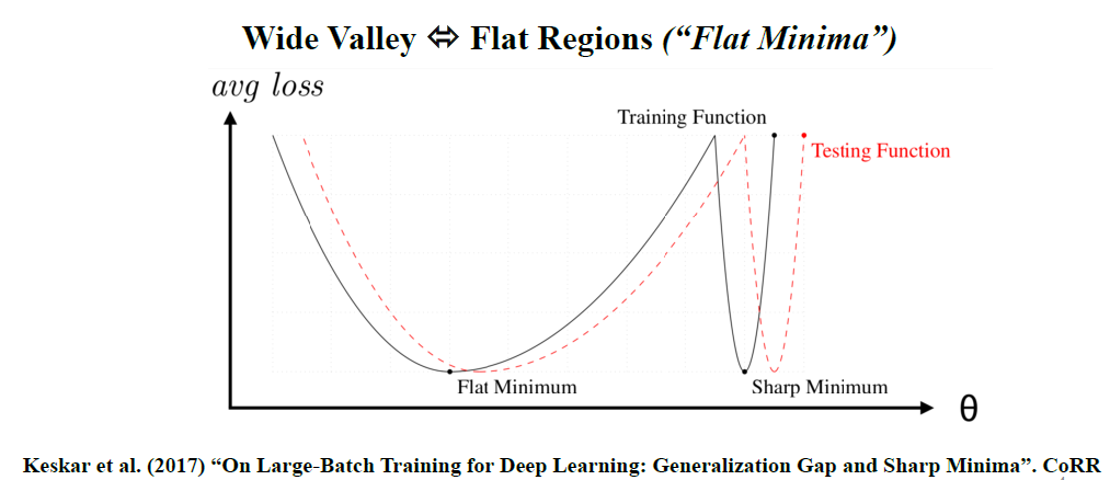
 

Figure 2
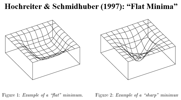
 

When we are in a region characterized as “flat minima”, the Loss Function changes more slowly. It is hypothesized that flat minima are “generalized” better. Thus, the motivation is to “bias” the objective function so that we end up with more “flat minima” (or “wide valleys”). This where the title of the paper partially comes from.

Now what do they mean by “generalized”? They refer to the “generalization error” (also known as the “out of sample error”). It is also refers on the concept “stability”, which I will discuss analytically.

Modify (Bias) the SGD

The modification (or biasing) of the SGD is by utilizing the concept of the local entropy. The were motivated by Baldassi et al. (2016) [2] who use “Local entropy as a measure for sampling solutions in constraint satisfaction problems”. 

The goal is to maximize (or minimize its negative) the following Equation 1:

Equation 1

This components of Equation 1 are as follows:

  1. F(x, \gamma) is the log partition function.
  2. The “depth” of the “valley” at a location \textbf{x} \in R^N
  3. The “flatness” is measured through the (local) entropy f(x^{'})
  4. The hyper-parameter  γ looks for “valleys” of specific “width”.

Intuition of Equation 1: “Bias” the optimization towards “wide (flat) valleys”.

The γ parameter

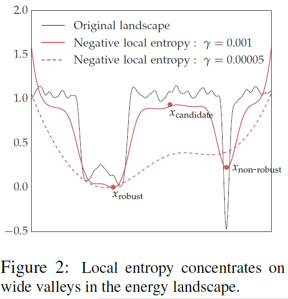
Let’s see the what γ does in practice. Figure 3 illustrates what happens to the loss function, the local entropy, when we increase γ. It becomes more “smooth”. Note that in Figure 3, the x-axis is the parameter space, the y-axis is the negative local entropy.

Figure 3
 

The Probabilistic Foundations

This is the point where we go deeper (learning sic).

The probabilistic foundations of local entropy lie in Equation 2:

Equation 2

This is a conditional probability with the following properties:

  1. For an \textbf{x} \in R^N parameter vector
  2. Consider a Gibbs-Sampling Distribution where:
    • f(x): is the energy landscape
    • β is the inverse “temperature” (see “Langevin dynamics”)
    • Z is a regularization term.

The reason we have these cryptic terms (“temperature”?) is because this is a mathematical modeling that is used in in physics, specifically the mathematical modeling of molecular systems. Not so cryptic.

Intuition: When \beta  \rightarrow  \infty , the probability distribution concentrates to the global minimum of \textbf{x}.

However, this is the gist: the authors want “flat regions”. Subsequently, they need a Modified Gibbs-Sampling Distribution, specifically the Equation 2 is modified into Equation 3:

Equation 3

Equation 3 is a conditional probability with the following terms:

  1. γ which “biases” toward  x .
  2. Large γ   \rightarrow   all the “mass” concentrates near x regardless of f(x^{'})  energy term (which measures “flatness” as discussed
  3. Small γ   \rightarrow f(x^{'}) dominates
  4. The authors set β=1, therefore β is a nuisance term.
  5. Instead, they focus on tuning γ

Revisiting the γ parameter: “scoping”

What Equation 3 tells us is that γ determines the “scope”. Specifically, in a neighborhood (region) around “x” (parameters):

  1. Large γ   \rightarrow   the proposed Stochastic Gradient Lavengin Dynamics (henceforth SGLD) updates in a smaller “neighborhood”.
  2. Smaller γ   \rightarrow     allow SGLD to explore in a  wider neighborhood (from x)

Why “Local” entropy?

Caveat: according to the authors local entropy is not equivalent to smoothing.

Local entropy means more weight on wide local minima even if they are shallower than the global minimum. As the authors stress “minimization of classical entropy would give us an optimal of x_{candidate} “.

ENTROPY-GUIDED SGD (SGLD)

By now you should know that SGLD and Entropy-Guided SGD are interchangeable. The authors use both terms to describe their method.

The ENTROPY-SGD is essentially an “SGD-inside-SGD” with an:

  1. Outer SGD updates the parameters
  2. Inner SGD estimates the gradient of local entropy

Furthermore the classical (vanilla) optimization problem is like this:

whereas an Entropy-SGD optimization:


Where Ξ is the data.

The  Gradient of Local Entropy

For \xi_{l_{i}} \in \Xi^{l} : randomly sampled mini batch of m samples:

Where for the computation of  \left\langle \Xi^{l} \right\rangle the current weights are fixed to x.

Moreover, the Gibbs Distribution of the Original Optimization is:

To this end, they utilize the “Langevin dynamics” (SGLD): an MCMC algorithm. The algorithm is as follows. However, there is a caveat in step 7 that is not properly addressed in the paper.
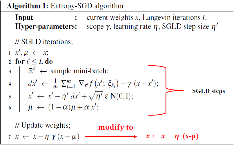
  • This algorithm is for 1 iteration:
  • ε: thermal noise
  • Fix: L, ε,   η
  • Step 7: As the authors stress, γ has to be tuned (scoping). Thus in practice the algorithm is modified as in Step 7.


The «Scoping» of γ

The scoping is formulated by the following framework:

  •  \gamma(t) = \gamma_{0} (1+\gamma_{1})^{t}
  • For t_{th} parameter update
  • The General strategy is:

1.Set \gamma_{0} very small

2.Large value for η

3.Set \gamma_{1}: such that the magnitude of the local entropy is comparable to SGD

THEORETICAL PROPERTIES

The authors show that:

  1. Entropy-SGD results in a smoother loss function
  2. and obtains better generalization

With two assumptions:

  1. The original f(x) is β-smooth
  2. no eigenvalue of the Hessian ^2 f(x) lies in [-2γ-c,c]
    1. For small c>0

The proof is based on a Laplace Transformation.
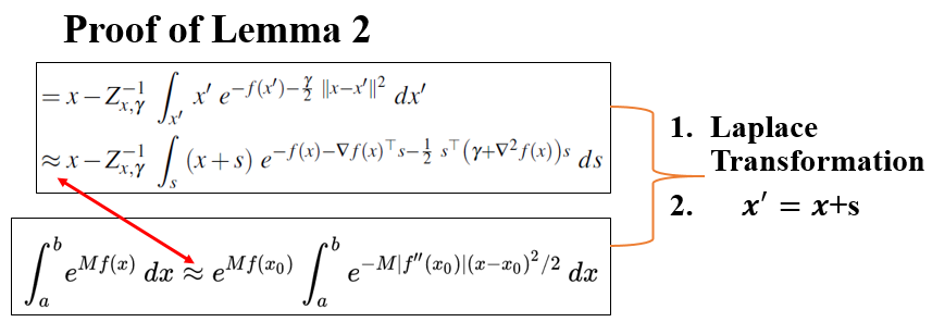
 

However the assumption regarding the bound is not as strong as the authors suggest. Moreover, the authors cite Hardt et al. (2015) who stress:

“This (assumption) is admittedly unrealistic [..] even if this assumption is violated to an extent before convergence happens.”

The authors are worried about the “stability” of the algorithm. Subsequently, they introduce the concept of an “ε-stable algorithm”, that places an upper bound to the algorithm:

Intuition: Under different samples of the general “population” the algorithm gives the same result, within little changes. The upper bound is derived by Theorem 3 and Lemma 2:

Experiments

The experiments were done as follows:

A. Two image classification datasets

  1. viz. MNIST
  2. CIFAR-10

B. Two Text prediction datasets

  1. viz. PTB
  2. text of War and Peace

The authors compute the Hessian at a local minimum at the end of training for the following networks:

  1. small-LeNet on MNIST:
  2. small-mnistfc on MNIST:
  3. char-lstm for text generation:
  4. All-CNN-BN on CIFAR-10

When a Hessian are very close to zero we have an almost flat at local minima. The authors compute the exact Hessian at convergence. The Entropy-SGD model is then compared to the SGD/ADAM. The results are demonstrated in the following Table that reports the the Error/Perplexity(%) per Epoch. The way the following table should be interpreted is that the model that performs better has a lower number of Epochs, for the same Error/Perplexity(%) per Epoch.
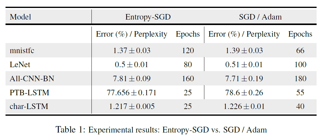
The authors also conducted a comparison between SGLD and Entropy-SGD, which is oddly reported in the Appendix, in the last page of the paper. This comparison was conducted for was for LeNET (300 Epochs) and ALL-CBB-BNN after (500 Epochs). The  test error on LeNet of 0.630\pm1 \% after 300 epochs and 9.890 \pm 11 \% on All-CNN-BN after 500 epochs. ARXIV

Assessment

The authors conclude that by using Langevin Dynamics to estimate “local entropy”: “can be done efficiently even for large deep networks using mini-batch updates”. One of the mane problems in the results is that no run-time speeds are reported. It is unclear whether the procedure’s increased computational cost is offset by the faster convergence. In addition, Baldassi et al. 2016 used a method called “Belief Propagation” to also estimate local entropy which is probably not given enough credit in this paper.

Notation

The paper uses Bra–ket notation (or Dirac notation) for probabilities:

https://quantummechanics.ucsd.edu/ph130a/130_notes/node107.html

References

[1] Chaudhari, Pratik; Choromanska, Anna; Soatto, Stefano; LeCun, Yann; Baldassi, Carlo; Borgs, Christian; Chayes, Jennifer; Sagun, Levent; Zecchina, Riccardo.  Entropy-SGD: Biasing Gradient Descent Into Wide Valleys. 2017

[2] Baldassi, C. Borgs, J. T. Chayes, A. Ingrosso, C. Lucibello, L. Saglietti, and R. Zecchina. Unreasonable effectiveness of learning neural networks: From accessible states and robust ensembles to basic algorithmicschemes. PNAS, 113(48):E7655–E7662, 2016.

[3] Nitish Shirish Keskar, Dheevatsa Mudigere, Jorge Nocedal, Mikhail Smelyanskiy, Ping Tak Peter Tang. “On Large-Batch Training for Deep Learning: Generalization Gap and Sharp Minima”. CoRR. 2017

[4] Hochreiter and J. Schmidhuber. Flat minima. Neural Computation, 9(1):1–42, 1997.

[6] M. Hardt, B. Recht, and Y. Singer. Train faster, generalize better: Stability of stochastic gradient descent. arXiv:1509.01240, 2015.



Lagrange dual

1. Lagrange dual problem: standard form, Lagrange dual function, and dual problem

First, we consider an optimization problem in the standard form:

minimize  f_{0}(x)

subject to  f_{i}(x) \leq 0, i = 1, …, m

 h_{i}(x) \leq 0, i = 1, …, p

with variable  x \in R^{n} , domain  D = \bigcap_{i=0}^{m} dom f_{i} \cap \bigcap _{i=1}^{p} dom h_{i} is nonempty. The optimal value is  p^{*} .

The idea of lagrangian duality is to take the constraints into account by augmenting the objective function with a weighted sum of the constraint functions.

Lagrangian  L: R^{n}\times R^{m} \times R^{p}\rightarrow R as:
L(x, \lambda , \nu ) = f_{0}(x)+ \sum_{i=1}^{m}\lambda _{i}f_{i}(x)+\sum_{i=1}^{p}\nu _{i}h_{i}(x),

with  dom L = D \times R^{m}\times R^{p},  \lambda _{i} as the Lagrange multiplier associated with the  i_{th} inequality constraint  f_{i}(x) \leq 0 and  \nu_{i} as the Lagrange multiplier associated with the  i_{th} equality constraint  h_{i}(x) = 0 .

Lagrange dual function is the minimum value of the Lagrangian.

For  \lambda \in R_{m}, \nu \in R_{p}
 g(\lambda, \nu) = inf_{x \in D} L(x, \lambda, \nu) = inf_{x \in D}(f_{0}(x) + \lambda _{i}f_{i}(x)+\sum_{i=1}^{p}\nu _{i}h_{i}(x))

If  \lambda \geq 0 , then  g(\lambda, \nu) \leq p^{*} .

Proof:

If  x\hat{~} is feasible and  \lambda \geq 0, then
 f_{0}(x\hat{~}) \geq L(x\hat{~}, \lambda, \nu) \geq inf_{x\in D}L(x, \lambda , \nu) = g(\lambda , \nu)
minimizing over all feasible  x\hat{~} gives  p^{*} \geq g(\lambda , \nu)

The dual problem: what is the best lower bound that can be obtained from the Lagrange dual function?

maximize  g(\lambda , \nu)
subject to  \lambda \geq 0
Optimal value is denoted as  d^{*}

2. Weak and strong duality

If   d^{*} \leq p^{*}, this property is called weak duality. The weak duality inequality holds when  d^{*} and d^{*} are infinite while If the equality  d^{*} = p^{*} holds then we say that strong duality holds.

3. Geometric interpretation of dual function and lower bound  g(\lambda) \leq p^{*}

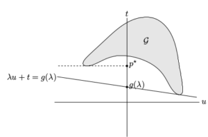
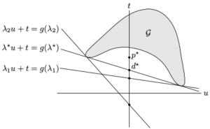
For a problem with one (inequality) constraint. Given λ, we minimize  ( \lambda, 1)^{T}(\mu, t) over G =\{(f _{1} (x), f _{0} (x)) | x \in D\} . This yields a supporting hyperplane with slope −λ. The intersection of this hyperplane with the u = 0 axis gives g(λ). Supporting hyperplanes corresponding to three dual feasible values of λ, i.e, optimum \lambda ^{\ast }\lambda ^{1 }, and \lambda ^{2 } . As shown in the figures, strong duality does not hold so the optimal duality gap p^{\ast }-d^{\ast } is positive.

4. Price or profit interpretation

Suppose the variable x denotes how an enterprise operates and  f_{0}(x) denotes the cost of operating at x, then  -f_{0}(x) is the profit made at the operating condition x.

Each constraint  f_{i}(x) \leq 0 represents some limit on resources (e.g., warehouse space, labor) or a regulatory limit (e.g., environmental). The operating condition that maximizes profit while respecting the limits can be found by solving the problem:

minimize f_{0}(x)

subject to  f_{i}(x) \leq 0, i = 1, …, m.

The resulting optimal profit is  - p ^{*} resulting optimal profit is  - p ^{*} .

Now imagine a second scenario in which the limits can be violated, by paying an additional cost which is linear in the amount of violation, measured by f_{i} .  Enterprise for the  i^{th} limit or constraint is  \lambda _{i}f_{i}(x) . Payments are also made to the firm for constraints that are not tight; if  f_{i}(x) \leq 0 represents a payment to the firm.

The coefficient  \lambda _{i} has the interpretation of the price for violating  f_{i}(x) \leq 0 ; its units are dollars per unit violation. For the same price the enterprise can sell any ‘unused’ portion of the  i^{th} constraint. We assume \lambda _{i} \leq 0 , i.e., the firm must pay for violations.

Reference

Boyd and Vandenberghe, Chapter 5–5.5 https://web.stanford.edu/~boyd/cvxbook/bv_cvxbook.pdf

Don’t Decay the Learning Rate, Increase the Batch Size

Background – 1 Stochastic gradient descent
A dominant optimization algorithm for deep learning. While SDG finds minima that generalize well, each parameter update only takes a small step in later training period because the learning rate would be very small.

Background – 2 Previous work
Previous works declare an optimum fluctuation scale g that can be found to maximize the test set accuracy (at constant learning rate). They introduce an optimal batch size that B << N, so that g = epsilon(N/B -1) where B means batch size and N means training set size.

Background – 3 Large batch training
Instead of decay the learning rate to make the optimization function converge, there is another approach that to increase the batch size. The advantages are that it can reduce the number of paras updates required and can also be parallelized well and reduce training time. There is a backward that when batch size increase, the test set accuracy often falls a little bit.

Reference – 1 Industry need for the training algorithm

Jonathan Hseu, Google Brain Scientist, is introducing the algorithm time complexity tolerance.

Reference – 2 Existing training approach speed on GPUComparing to the existing work on GPU, this paper can train ResNet-50 on ImageNet to get 76.1% accuracy in 30 mins, by making the full use of the characteristic of TPU.
Main content – 1 Existed problem
When one decays the learning rate, one simultaneously decays the g. However, the learning rate is not the necessary factors to decays the g and make the function converge.

Main content – 2 Solution
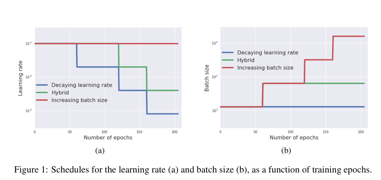
Do increase the batch size during training instead of decaying the learning rate. When learning rate wants to drop by alpha, it increases the batch size by alpha.

Main content – 3 Advantage
First, This approach can achieve a near-identical model performance with the same number of training epochs. Second, it significantly reduces the parameter updates in the training process. Third, it doesn’t require any fine-tuning process.

Main content – 4 Further Enhancement
After achieving the same quality of result with the learning rate decay approach, the batch size increase approach is also able to further reduce the number of para updates by further increasing the learning rate, scaling B that proportional to epsilon or increasing the momentum coefficient and scale B that proportional to 1/(1-m).

Main content – 5 Consequent
It successfully trains an Inception-ResNet-V2 on ImageNet under 2500 para updates using batches of 65536 images and gets 77% accuracy. It successfully trains a ResNet-50 on ImageNet to 76.1% accuracy in 30 mins.

Main content – 6 Contribution
First, it shows the quantitative equivalence of increasing the batch size and decaying the learning rate. Second, it provides a straightforward pathway towards large batch training.

Result analysis – 1Figure 1 shows an example that how the learning rate and batch size change in the different algorithms. For the blue line decaying learning rate, the learning rate is reduced in the training process (number of epochs increase) but the batch size is always constant. For the red line increasing batch size, the batch size is increased in the training process (number of epochs increase) but the learning rate is always constant.
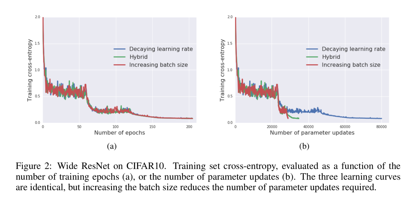
Result analysis – 2Figure 2 shows that the increasing batch size approach can achieve a qualitatively equivalent result than the decreasing learning rate approach. However, it only needs around 1/3 training updates.

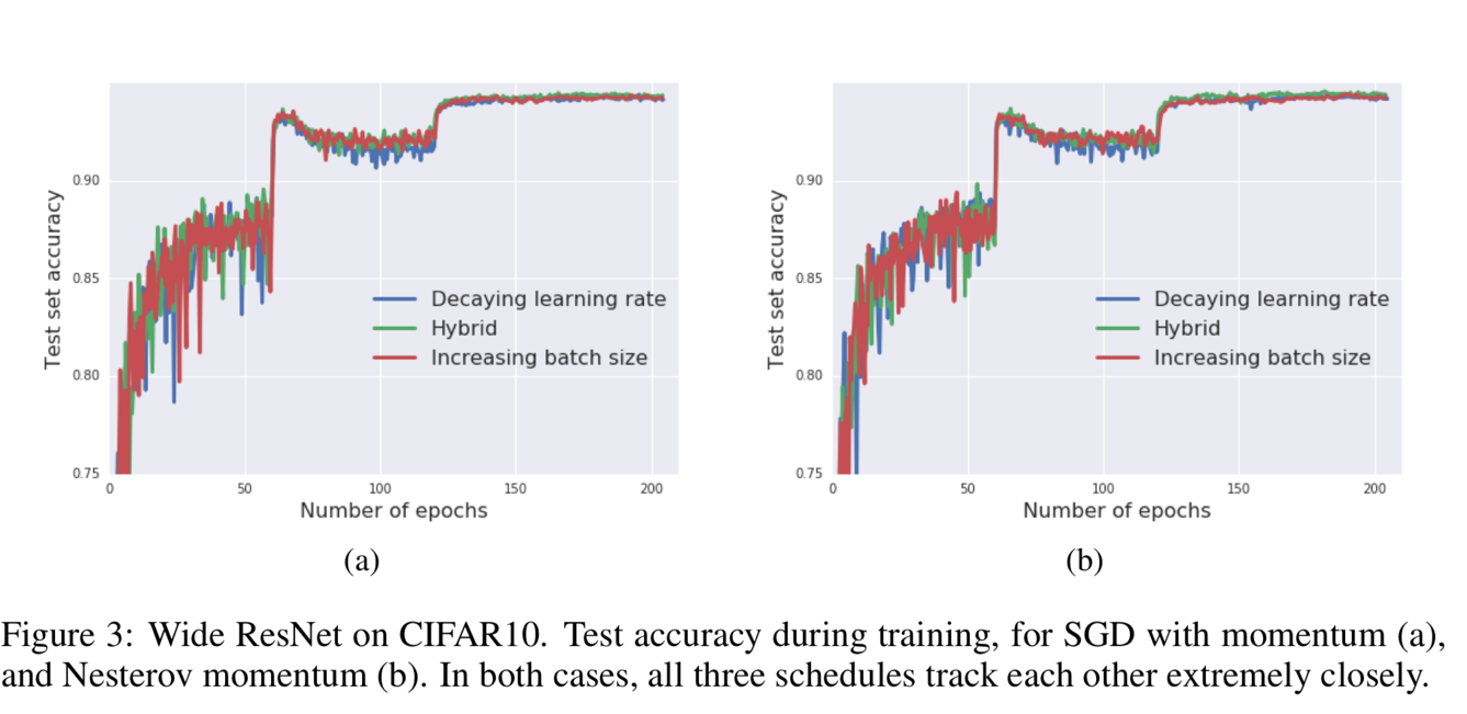
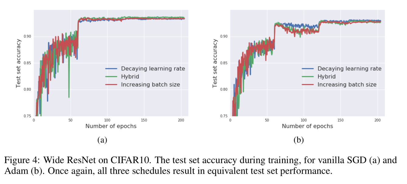
Result analysis – 3 & 4Figure 3 and Figure 4 show that the batch size increasing approach can be applied to many different optimization algorithms, like SGD with momentum, Newterow momentum, vanilla SGD and Adam.
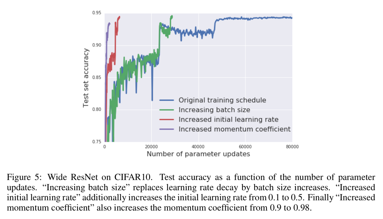
Result analysis – 5Figure 5 shows the truth that after achieving the same quality equivalent of result with the learning rate decay approach, the batch size increase approach is also able to reduce the number of para updates further. Blue: original learning rate decaying method; Green: batch size increasing method; Red: batch size increasing method + further increase initial learning rate; Purple: batch size increasing method + further increase initial learning rate + further increase momentum coefficient.

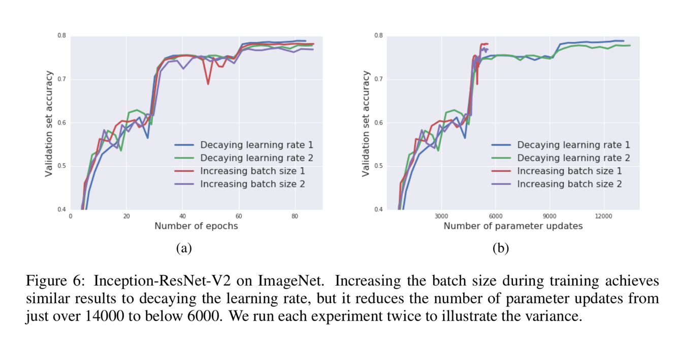
Result analysis – 6Figure 6 proves the validity and reproducibility of this algorithm by conducting the experiments many times.
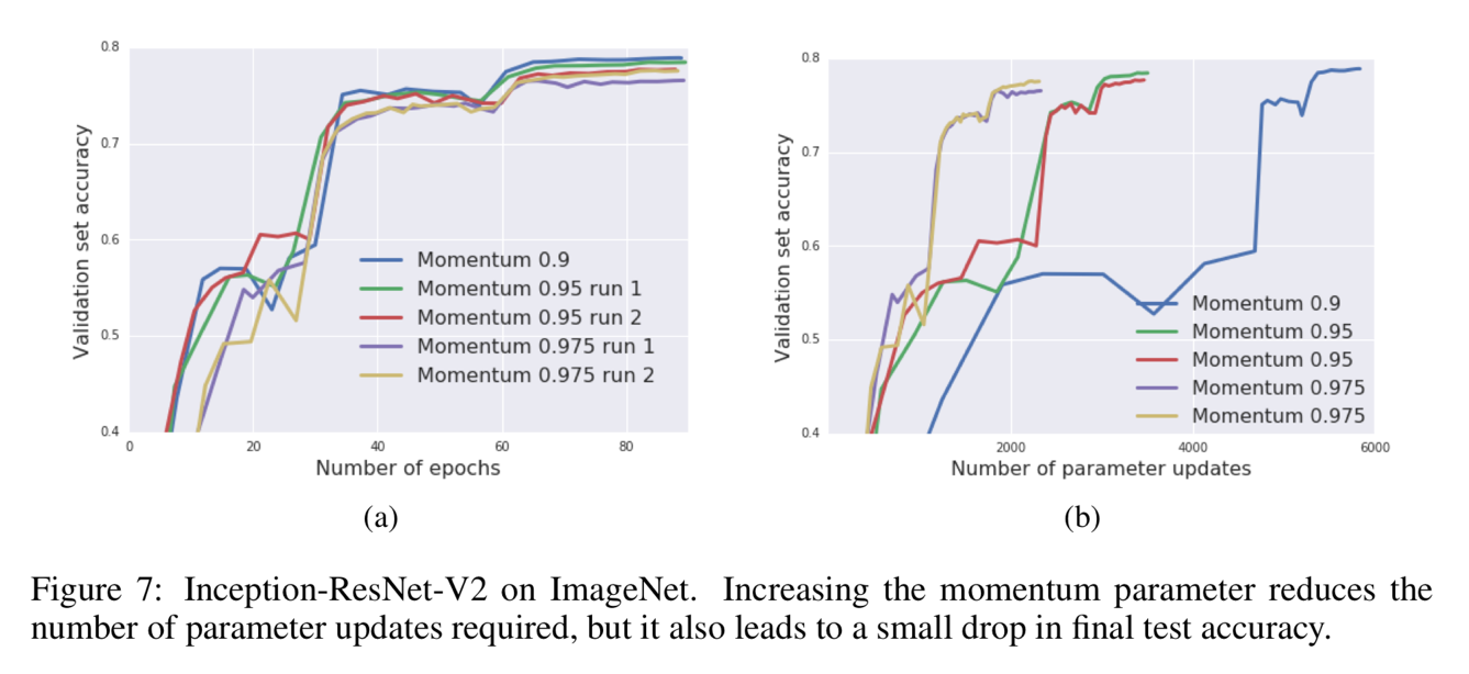
Result analysis – 7Figure 7 shows that the influence of momentum coefficient that increasing the momentum can reduce the update times as well as reduce the training time consuming but can let the accuracy fall a little bit.

Backpropagation is not just the chain rule

Author: Jiamin Wang and Spencer Jenkins

Motivation

Basically, machine learning problem is about function approximation. If we have datasets (x, y), is the variables and is the response, and we want to fit some function f, parameterized by some parameter vector θ, f(x), to predict y. In neural network framework, the fitted function is usually nonlinear. We can define the loss function measuring how well function f’s prediction. Finally, some local optimization algorithm can be employed to minimize the loss function. 

minimize

If we want to calculate the minimum of loss function, we need compute the derivative of loss function with respect to the parameter .

But the loss function obtained from neural network model is very large, so that we can’t generally write it down in any closed-form. There is one example provided in the blog:

f(x)=exp(exp(x) + exp(x)^2) + sin(exp(x) + exp(x)^2)

If we compute the derivative using symbolic differentiation,which the ‘flat’ version of this function.  The math expression show:

df/dx=exp(exp(x)+exp(x)^2)(exp(x) +2exp(x)^2) + cos(exp(x) +exp(x)^2)(exp(x)+2exp(x)^2)

It isn’t too hard to explicitly write down this equation. However the actual loss function is even much more complicated, and the derivative will explode.

Automatic differentiation

In a smart way, we can use the automatic differentiation(autodiff), which has two modes forward and reverse. In neural nets framework, reverse mode of autodiff is also called back propagation. Both of these two modes need to calculate f(x) and become slow when the input variable is in high dimension.

What is autodiff, autodiff is compute the derivative by defining some intermediate variables as shown below:

a=exp(x)

b=a^2

c=a+b

d=exp(c)

e=sin(c)

f=d+e

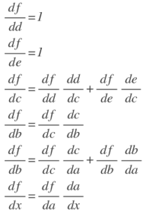
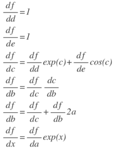
It is convenient to draw the graph to illustrate the relationship between all the intermediate variables. We can work backwards to calculate the derivative of f with respect to each variable by the chain rule.


In this way, we can compute the derivative of each variable and make use of the derivatives of the children of that variable.

  • The general formulation of forward propagation. Variable are the input and are the intermediate variables, is the final value. The functionsare defined as the elementary functions evaluated on the ‘parents’ Pa(i) of variable i. The formulation of forward propagation is

For i=n+1, n+2….N:

  • The general formulation of backward propagation. The derivative of function f with respect to the final value

For i = N-1, N-2,….1:

Advantages of Autodiff

Space complexity: Autodiff has fewer thing to memorize. The rules for transforming the code for a function into code for the gradient are really minimal.

Time complexity: The program for the gradient has exactly the same structure as the function, which implies that we have the same runtime.

Autodiff by the method of Lagrange multipliers

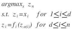
Intermediate variables are the equality constraint in the optimization problem. Blog example can be written in this constraint form:

argmax f

s.t.  a=exp(x)

b=a^2

c=a+b

d=exp(c)

e=sin(c)

f=d+e

The general formulation

  • Input variables: 
  • Intermediate variables:the term is the parents of i.
  • Output variable(): we assume the programs have a singled scalar output variable  which represents the quantity we want to maximize.

The standard way to solve the constrained optimization is to converts the constrained optimization problem into an unconstrained formula with parameters , called Lagrange multipliers.

The really interesting result in this blog post comes from applying the method of Lagrange multipliers to the constrained optimization form of our problem as shown above. By introducing additional variables (known as Lagrangian multipliers), we can turn our problem into an unconstrained optimization problem which takes the following form:

We call the above form the Lagrangian. To optimize our Lagrangian, we take its gradient and set it equal to zero. We then solve for our Lagrange multipliersand our intermediate variables .

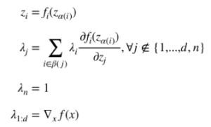
The original blog post does a good job of deriving the results of this optimization, so we won’t go into too much detail on the process. The main results, however, are summarized below:

There are a few interesting things to observe from the results of the Lagrangian method. First, we can see that satisfying the constraints on our intermediate variables can be interpreted as the feedforward step in backpropagation. Second, we can see that the result we get for our Lagrangian multipliers is of the same form as what we get during backpropagation. We are summing all λ that directly depend on j, scaling each by the derivative that relates i and j. This is an equivalent operation to determining our δ terms in backpropagation. Lastly, we see that we can solve for our Lagrange multipliers and our intermediate variables by performing back-substitution. We cannot, however, obtain a closed-form solution for our input variables. We can only solve for  and thus obtain the gradient of our original function. To solve for the input variables, we will have to perform something like gradient ascent.

The author goes on to briefly describe how cyclic constraints could also be handled by this approach. The feedforward procedure becomes more difficult and a linear solver is required to determine the Lagrangian multipliers, but the procedure essentially stays the same.

The main benefit of thinking about backpropagation in the Lagrangian sense is the ability to apply constrained optimization algorithms to our problem. The author doesn’t go into much detail on use cases and benefits for this approach, but it isn’t hard to imagine that considering other algorithms might prove useful given certain problems. The connection between backpropagation and the method of Lagrange multipliers is more than just a curiosity.

As a final note, we found the following paper helpful in understanding the ideas presented in the blog post: A Theoretical Framework from Back-Propagation (LeCun, 1988). It presents the same idea as the blog post, organized in a very similar manner. The notation in this paper is more closely related to how backpropagation is typically formulated (the blog post deals with a slightly more general form), so the connection between backpropagation and the method of Lagrange multipliers might become more clear after reading this resource.

Training Neural Networks Without Gradients : A Scalable ADMM Approach

Training Neural Networks Without Gradients : A Scalable ADMM Approach

Introduction


Many research have been conducted in training Neural Networks. Most common method is using stochastic gradient method combine with backpropagation. The paper notice the weakness of this conventional method and suggest their proposed method which is using alternating direction method of multipliers (ADMM) with bregman iteration.

Why we need proposed method ?

Weakness of conventional optimization rely on stochastic gradient method in Neural Networks is that they do not scale well to large number of cores in a cluster setting. Also as the method is gradient-based, there are problems with convergence such as saturation effect or stock in local optimal point or vanishing gradients. In addition, backpropagation does not easily parallelize over layers.

To solve these problems proposed method separate the objective function at each layer of a neural network into two terms.

First term is measuring the relation between the weights and the input activations. Second term is containing the nonlinear activation function.

This structure allows the weights to be updated without the effects of vanishing gradient and stock in local optimal. Also form of the objective allows the weights of every layer to be updated independently, enabling parallelization over layers.

By separating the objective function, proposed method decomposes with the sequence of minimization sub problems which is ADMM scheme, and it can solve globally & closed form. Also, combining bregman iteration, the solution of proposed method could be stable.

In addition proposed method exhibits linear scaling when data is parallelized across cores.

Notation

Let’s define notation, before checking the model of proposed method.

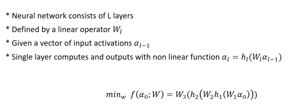
Neural network consists of L layers and defined by a linear operator W

objective function is shown as above.

Model of proposed method

Now, let’s check the model.


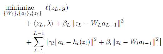
we want to minimize loss function. Two constraint is corresponding to the constraint that I explained above. To make unconstrained problem, they use penalty term .

Proposed method use lagrange multiplier only related with objective term. Thus the model became as below.

Compare to classical ADMM which use lagrange multiplier to all the constraint, the proposed method only apply to objective term.

This is because as proposed scheme involves more than two coupled variable blocks and non smooth function, it lies outside the scope of known convergence results for ADMM. Thus they cannot apply to all constraints but just objective term and this part is related with bregman iteration in proposed method. The convergence of bregman iteration is well understood in the presence of linear constraints.

Before checking bregman iteration, let’s see the sub-problem which is the property of ADMM scheme in proposed method.

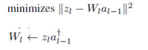
There are several parameters to update in neural network. Weight, input activation and output activation and lagrange multiplier are parameter to be updated.

  • Weight update (LSE)

  • Activation update (LSE)

  • Output update

Sub problems of updating weight and activation are easy. It can be solved in LSE.

Output update is challenging separable updating in ADMM scheme. However as entries in Z_{l} are decouple, the problem can be decomposes into solving a large number of one-dimensional problems, one for each entry in Z_{l}.

Bregman iteration

Now let’s check the update of largrage multiplier and bregman iteration. We already check that the reason proposed method used bregman iteration.

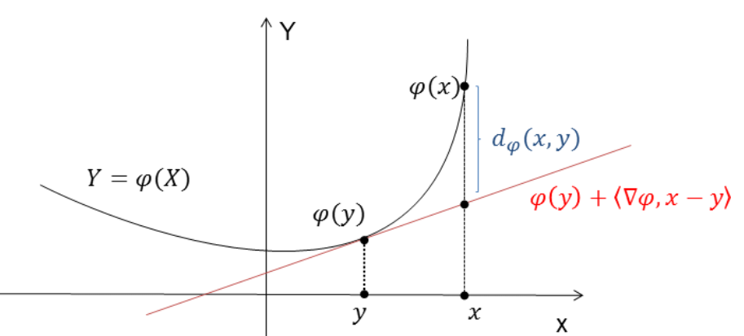
Bregman distance with a convex function E at the point v is 

Geometrically we can interpret as below

which is the distance between function value and tangent line.

Starting from minimize convex function E and linear constraint H and penalty coefficient lambda, bregman iteration perform as below.

Thus, we checked that how does the subgradient is updated in bregman iteration.

Let’s come back to our problem.

with respect to Z_{l} we can obtain

we can check above equation is identical to update equation of subgradient in bregman iteration. Thus, we could interpreted as largragian multiplier as subgradient in bregman iteration.

I think this is the reason the largrangian multiplier is applied to only objective term. To use bregman iteration, they need the largrangian multiplier term related with objective function to update as subgradient in bregman iteration.

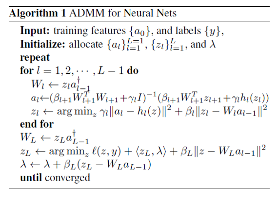
Below is the algorithm for proposed method what I mentioned until now.

Implementation & Data parallel

  • Distributing the algorithm across N worker nodes. (CPU parallel computation)
  • Different nodes store activations and outputs corresponding to different subsets of training data.
  • To start good initial value for converge, they used proposed method by running several iterations without largrangian multiplier updates at first.
  • set large value in penalty coefficients.
  • Training data is binary class label
  • Loss function is hinge penalty form which is convex function.

Experiment Result

  • They compare the proposed method with gradient-based method with GPU computation which is conjugate gradients, SGD and L-BFGS.

SVHN DATA

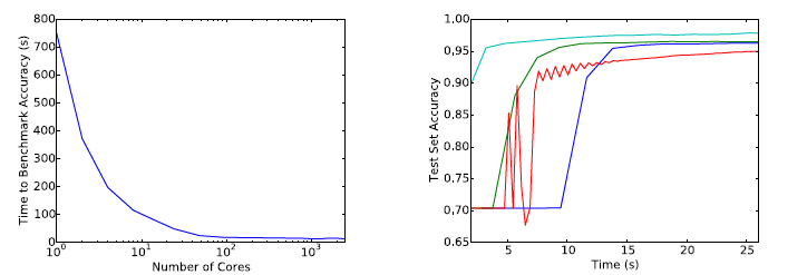
First, they focus on the problem posed by the SVHN dataset. For this dataset, they optimized a net with two hidden layers of 100 and 50 nodes and ReLU activation functions. The data is relative small and easy to train.

Above is the result. First graph shows that time required for proposed method to reach 95% test accuracy vs number of cores. We can check the advantages of scaling of proposed method. Second graph shows test set predictive accuracy as a function of time in seconds for each method. We can not say that proposed method have outperformance to other method.

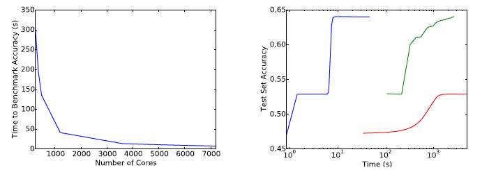
Second, they focus on Higgs dataset which is relative larger and difficult to train. They optimized a simple network with ReLU activation function and a hidden later of 300 nodes.

Above is the result. From the first graph, we can still check the scalability of the proposed method. From the second graph, the proposed method ( blue ) have outperformance in this dataset than the methods based on gradient with GPU computation.


Conclusion

  • They present a method for training neural networks without using gradient steps.
  • Proposed method avoid many difficulties of gradient method.
  • Performance of the proposed method scales linearly up to thousands of cores.
  • Proposed approach out-perform other methods on problems involving extremely large datasets.

Federated Optimization: Distributed Machine Learning for On-Device Intelligence

Introduction

Standard machine learning approaches require centralizing the training data on one machine or in a datacenter. This work introduces an additional approach: Federated Learning, which leaves the training data distributed on the mobile devices, and learns a shared model by aggregating locally computed updates via a central coordinating server.

State-of-the-art optimization algorithms are typically inherently sequential. Moreover, they usually rely on performing a large number of very fast iterations. However, the round of communication is much more time-consuming than a single iteration of the algorithm, which lead to the development of novel algorithms specialized for distributed optimization.

Problem Formulation

This model proposed in this paper are considering the problem of minimizing an objection function that has the form of a sum, which is like this:

The examples for this kind of problem structure covers:

The Setting of Federated Optimization

Since communication efficiency is of utmost importance, algorithm for federated optimization follow the following characteristics.

Massively Distributed:

Data points are stored across a large number of nodes K. In particular, the number of nodes can be much bigger than the average number of training examples stored on a given node (n/K).

Non-IID:

Data on each node may be drawn from a different distribution; that is, the data points available locally are far from being a representative sample of the overall distribution.

Unbalanced:

Different nodes may vary by orders of magnitude in the number of training examples they hold.

Federated Learning

Federated Learning enables mobile phones to collaboratively learn a shared prediction model while keeping all the training data on device, decoupling the ability to do machine learning from the need to store the data in the cloud. This goes beyond the use of local models that make predictions on mobile devices by bringing model training to the device as well.

It works like this: your device downloads the current model, improves it by learning from data on your phone, and then summarizes the changes as a small focused update. Only this update to the model is sent to the cloud, using encrypted communication, where it is immediately averaged with other user updates to improve the shared model. All the training data remains on your device, and no individual updates are stored in the cloud.

Distributed settings and desirable algorithmic properties

We consider two distributed settings in this work. On a single machine, we compute the execution time as

where  is the number of iterations algorithm A needs to converge to some fixed ε accuracy.is the time needed for a single iteration.

On natural distributed machines, the execution time includes the communication overhead  in a single iteration; c >> .

Desirable algorithmic properties for the non-IID, unbalanced, and massively-distributed setting are:

Property (A) is valuable in any optimization setting. Properties (B) and (C) are extreme cases of the federated optimization setting (non-IID, unbalanced, and sparse), whereas (D) is an extreme case of the classic distributed optimization setting (large amounts of IID data per machine). Thus, (D) is the least important property for algorithms in the federated optimization setting.

SVRG algorithm on a single node

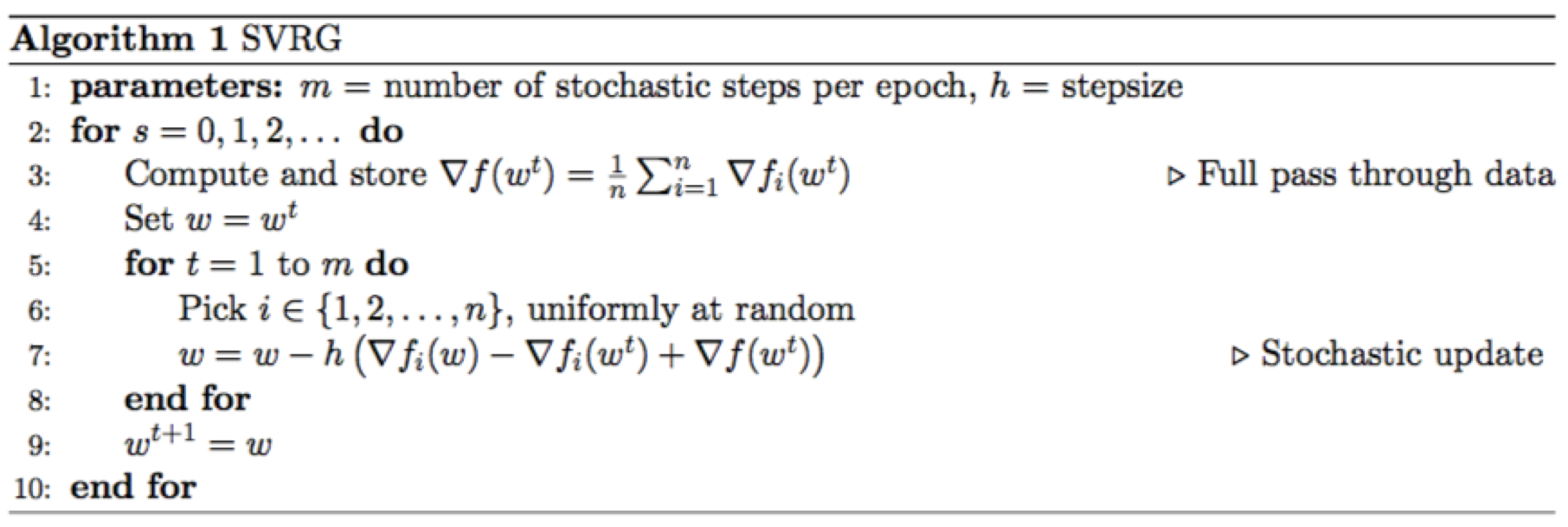
The Central idea is the algorithm evaluates two stochastic gradients,∇fi(w) and ∇fi(wt) to estimate the change of the gradient of the entire function between points wt and w, namely ∇f(w)− ∇f(wt).

Under a distributed setting, we modify the objective as below:

The original problem formulation is  If we define  then 

Therefore, the objective is changed to

Distributed Approximate Newton algorithm (DANE)

The main idea of DANE is to form a local subproblem, dependent only on local data, and gradient of the entire function — which can be computed in a single round of communication.

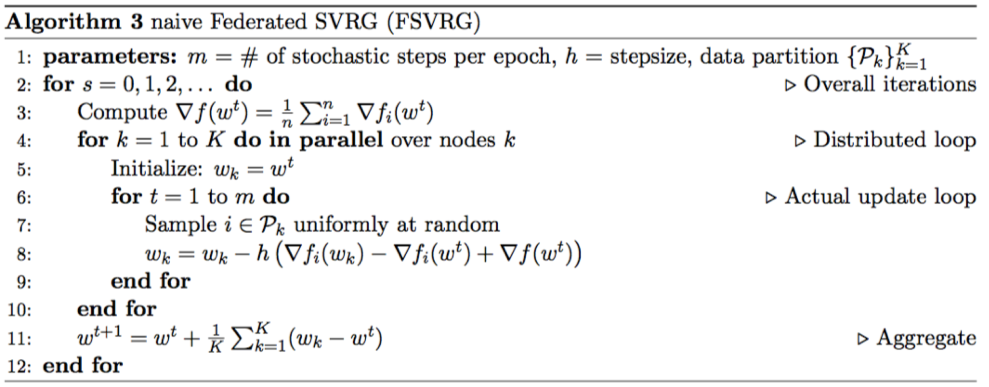
Naive Federated SVRG

This proposition proves the effectiveness of the naive federated SVRG algorithm. However, this algorithm is inherently stochastic, and is valid under identical sequence of samples. This work further improves this algorithm to get the federated SVRG.

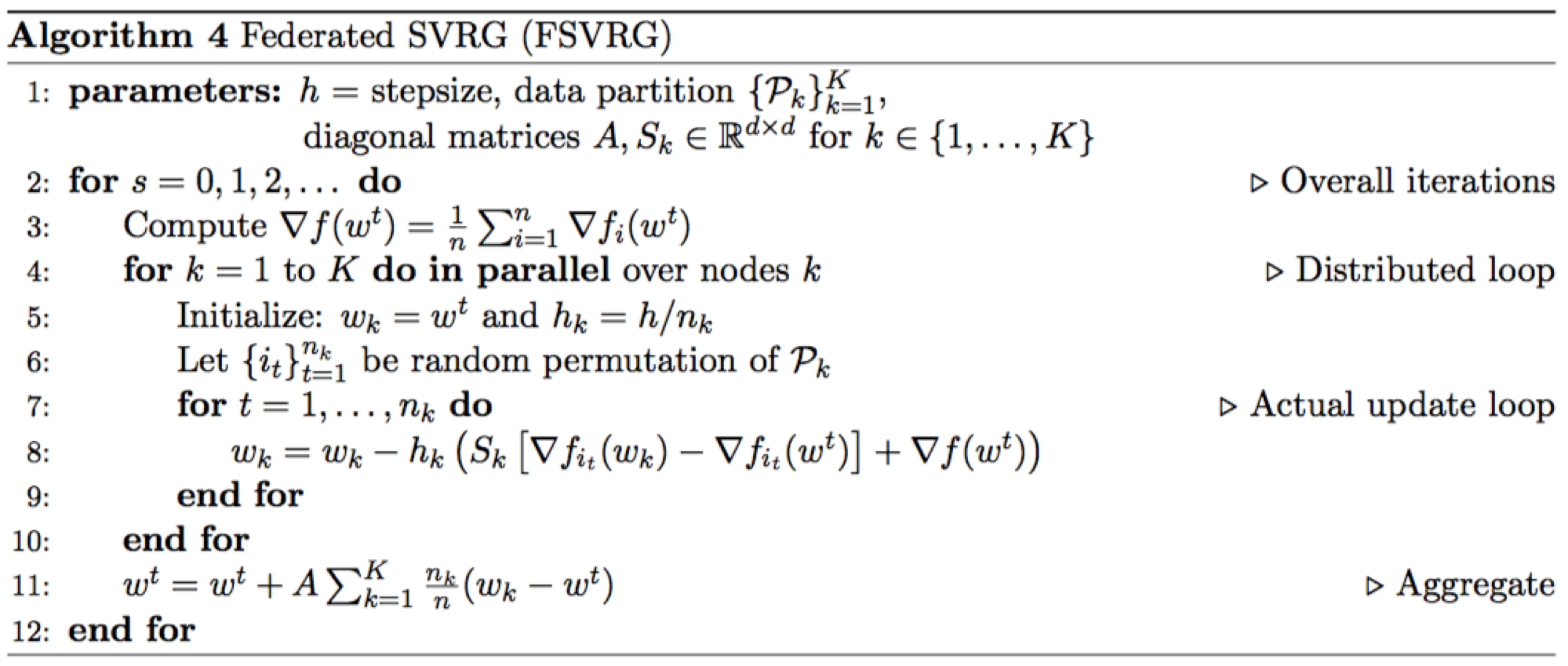
The Federated SVRG

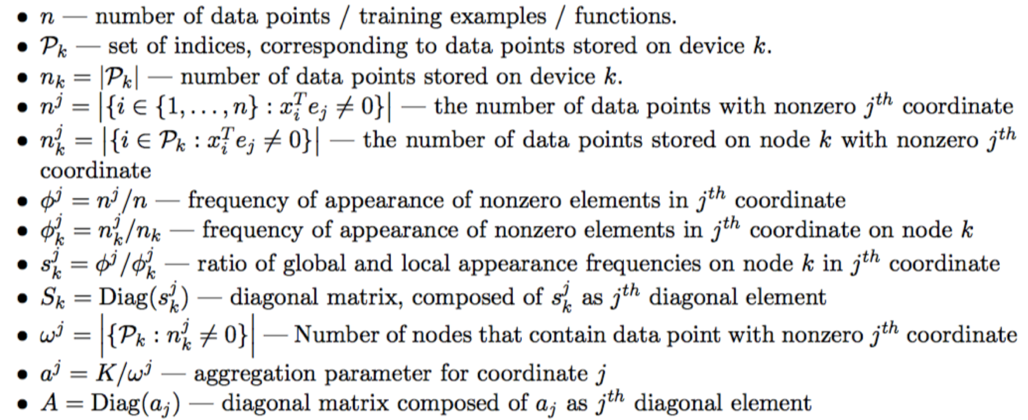
The notations used in this work are summarized below:

Federated SVRG improves from naive federated SVRG from four parameters:

Since the local data sizes, nk, are not identical, so setting the stepsize hk inversely proportional to nk, making sure each node makes progress of roughly the same magnitude overall.

If K is more than 1, the values of Gk are in general biased estimates of ∇f(wt).

This motivates the aggregation of updates from nodes proportional to nk, the number of data points available locally.

Because of the un-even distribution of nonzeros for a particular feature,

repeatedly sampling and overshooting the magnitude of the gradient will likely cause the iterative process to diverge quickly. So we scale stochastic gradients by diagonal matrix Sk.

If a variable appears in data on each node, we are going to take average. However, the less nodes a particular variable appear on, the more we want to trust those few nodes in informing us about the meaningful update to this variable — or alternatively, take a longer step. Hence the per-variable scaling of aggregated updates.

Experiments

They provide results on a dataset based on public Google+ posts, clustered by user — simulating each user as a independent node.

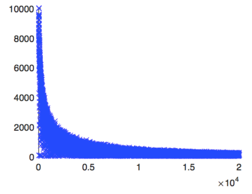
The following figure shows the frequency of  different features across nodes. In particular, over 88%
of features are present on fewer than 1000 nodes, which simulate the structure of distribution of the sparsity pattern.

Figure 1: Features vs. appearance on nodes. The x-axis is a feature index, and they-axis represents the number of nodes where a given feature is present.

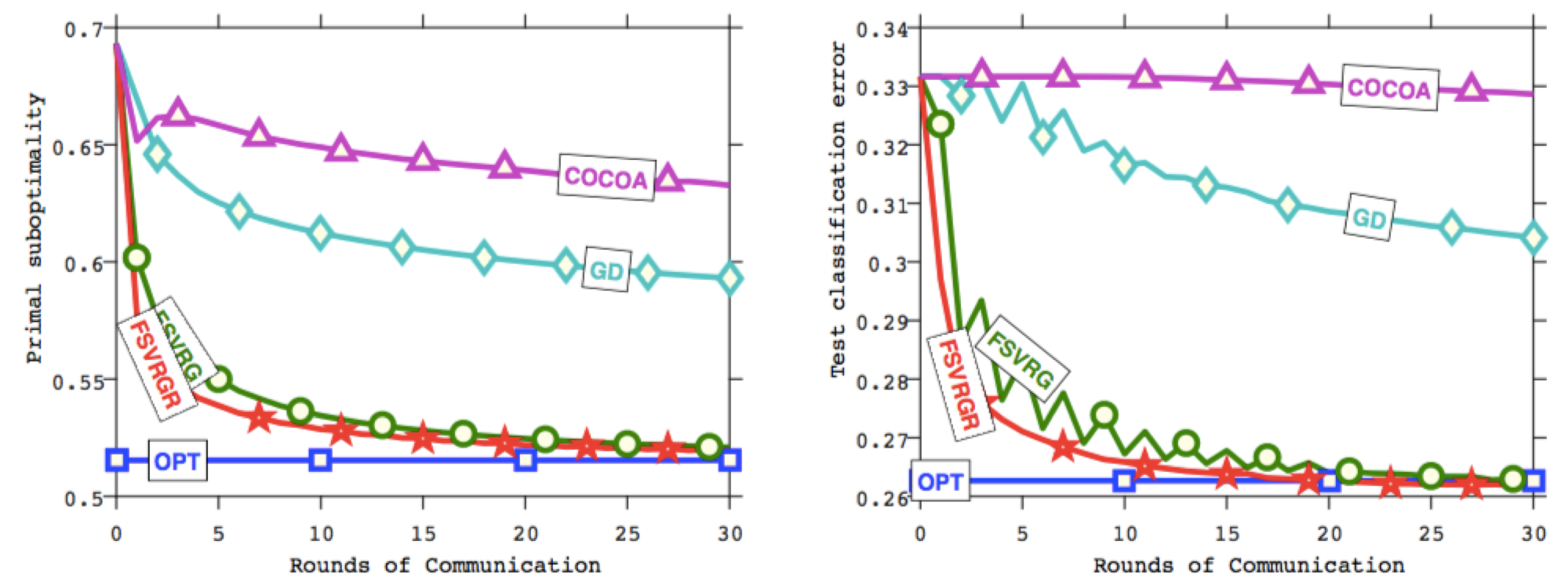
Figure 2: Rounds of communication vs. objective function (left) and test prediction error (right).

Figure2 show that FSVRG, converges to optimal test classification accuracy in just 30 iterations. Since the core reason other methods fail to converge is the non-IID data distribution, the experiment test the FSVRGR algorithm with data randomly reshuffled among the same number of nodes, which illustrate the algorithm is robust to challenges present in federated optimization.