yufengma

Identifying the Saddle Point Problem in High-dimensional Non-convex Optimization (Mukund)

Non-Convex Optimization

Non-convex optimization problems are any group of problems which are not convex (concave, linear etc.). These non-convex optimization problems are difficult to solve because non-convex functions have potentially many local minima and finding the global minima among all the local minima is hard. For this reason, solving such optimization problems are at least NP-Hard. Other reasons which make optimizing non-convex problems are

the presence of saddle points
very flat regions exhibited in the curvature
the curvature of such functions can be widely varying.

Traditionally, methods like Gradient descent, Newton Methods which are used to solve convex optimization problems are used to solve non-convex optimization problems as well.

Saddle Points

Given a function f, a critical point is defined as the point in the function where the derivative of f becomes 0. Typically, critical points are either maxima or minima (local or global) of that function. Saddle points are special type of critical points where the slope becomes 0, but are not local extremum in both axes.

For example, in the graph ${z = x^2 - y^2}$ , the point (0,0) is the saddle point because the gradient at (0,0) is 0, but the point in neither a local maxima not a local minima.

At this point, let us talk a bit more about critical points. The curvature of the function surrounding these critical points can tell us a lot about these critical points itself. The curvature of the function can be evaluated using the Hessian at these points. The eigen values of the Hessian at the critical point can describe the critical point.

If the eigen values are all non-zero and all positive, then the critical point is local maxima
If the eigen values are all non-zero and all negative, then the critical point is local minima
If the eigen values are all non-zero and mix of both positive and negative values, then the critical point is saddle point
If the Hessian matrix is singular, then the critical point is a degenerate critical point

Saddle Point Problem in High Dimensional Non-convex Problems

When a non-convex error function has a single scalar variable, there might be a lot of local maxima and local minima in the function but there is very negligible probability of occurrence of a saddle point. Whereas error functions with N scalar variables are likely to have more saddle points than local minima. In fact, as the dimensionality (N) increases, the number of saddle points increases exponentially. There have been many studies to prove this point. When dealing with high dimensional non-convex problems, which is the case with real world problems, we have to deal with these saddle points. The traditional methods like gradient descent and Newton methods perform poorly in presence of these saddle points. The gradient descent methods are repelled away from these saddle points, but the convergence is painfully slow. Whereas the Newton methods in an effort to speed up convergence, get attracted to these saddle points and do not converge on the local minima.

Dynamics of Optimization Algorithms around Saddle Points

To better understand the difficulty of existing optimization algorithms for high dimensional non-convex problems, it is helpful to understand how these algorithms behave near saddle points during the optimization process.

We can re-parameterize the critical points using the Taylor expansion so that they can be locally analysed. The Taylor expansion can be given as:

$f(\theta^* + \Delta \theta) = f(\theta^*) + \frac {1}{2} \sum_{i=1}^{n} \lambda_{i} \Delta v_{i}^2$

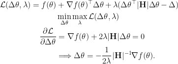
The step size that the gradient descent method uses is $-2 \lambda_i \Delta v_i$ . A step of the gradient descent method will always move in the right direction around the saddle point. If the eigen value is positive, we move towards that point in the direction of the negative curvature and hence the gradient descent method will always move away from the saddle points. The problem with gradient descent is the step size. Because gradients are proportional to corresponding eigenvalues, eigenvalues dictates how fast we move in each direction. If there is a large discrepancy in eigenvalues, the gradient descent will take very small steps.†It might take a very long time to move away form the critical point, if the critical point is a saddle point, or to the critical point if it is a minimum.

The Newton method rescales the gradients in each direction with the inverse of the corresponding eigenvalue. The step size used in the Newton method is $- \Delta v_{i}$ . If the eigenvalue is negative, the Newton method moves in the opposite direction to the gradient descent method due to the rescaling. This results in moving in the wrong direction around the saddle points and Newton methods instead of escaping the saddle point converge on them.

The trust region is a second order method, where the step size taken is $- ( \frac {\lambda_i} {\lambda_i + \alpha} ) \Delta v_i$ . This speeds up the convergence significantly and this method moves in the same direction as the gradient descent method, thus escaping the saddle points. It can also suffer the drawback of slow convergence sometimes if $\alpha$ is too large.

Attacking the Saddle Point Problem in High-dimensional Non-convex Optimization (Yufeng)

Problems with Stochastic Gradient Descent (SGD) and Newton Method

Based on our previous analysis, we know that saddle points are ubiquitous in high dimensional non-convex optimization problems. However, we are still uncertain about how modern optimizers would behave around these saddle points. Specifically, we would like to focus on Stochastic Gradient Descent (SGD) and Newton method here.

Suppose we have a function $f(\theta)$ , in which $\theta$ stands for the whole parameters of a model that we want to optimize. Besides, we have a saddle point $\theta^*$ . Then we may approximate $f(\theta)$ around this saddle point using second-order Taylor expansion by

$f(\theta^* + \Delta\theta) = f(\theta^*) + \nabla f(\theta^*)^\top \Delta\theta + \frac{1}{2} (\Delta\theta)^\top \mathbf{H} \Delta\theta.$

Since a saddle point is also a critical point, the second first-order term can be cancelled with $\nabla f(\theta^*)$ being a $\mathbf{0}$ vector. Now let’s reparametrize $\Delta\theta$ based on how it changes along orthonormal eigenvector directions of the Hessian matrix $\mathbf{H}$ , i.e., $\mathbf{e}_1, \dots, \mathbf{e}_{n_\theta}$ . Here $n_{\theta}$ represents the number of eigenvectors for $\mathbf{H}$ . Correspondingly, we also have eigenvalues $\lambda_1, \dots, \lambda_{n_\theta}$ . Then the movement along eigendirections can be formulated as

$\begin{aligned} \Delta \mathbf{v} &= \left[ \begin{array}{c} e_1^\top\\ \vdots\\ e_{n_\theta}^\top \end{array} \right] \Delta\theta \end{aligned}.$

Since a Hessian matrix should be both real and symmetric, with orthonormal eigenvectors, it can be represented by

$\mathbf{H} = [ e_1, \dots, e_{n_\theta} ] \Lambda \left[ \begin{array}{c} e_1^\top \\ \vdots \\ e_{n_\theta}^\top \end{array} \right],$

where $\mathbf{\Lambda}$ is the matrix with eigenvalues on the diagonal. Therefore, our Taylor expansion approximation can be expressed as:

$\begin{aligned} f( \theta^* + \Delta\theta ) &= f(\theta^*) + \frac{1}{2} (\Delta\theta)^\top \overbrace{ [ e_1, \dots, e_{n_\theta} ] \mathbf{\Lambda} \left[ \begin{array}{c} e_1^\top \\ \vdots \\ e_{n_\theta}^\top \end{array} \right] }^{\mbox{ Orthonormal }} \Delta\theta \\ &= f(\theta^*) + \sum_{i=1}^{n_\theta} \lambda_i \Delta\mathbf{v}_i^2 \end{aligned}.$

Based on the above reparametrization, we can now go forward with how SGD and Newton method stroll around the saddle point $\theta^*$ . First for SGD, the movement along a specific eigenvector $e_i$ is defined as

$\mathbf{m}_i = -\lambda_i \Delta\mathbf{v}_i.$

It’s worth mentioning that we are actually moving along the correct direction here. However, with $\lambda_i$ scaling before $\Delta\mathbf{v}_i$ , eigenvalues of different magnitudes will result in different step sizes along eigenvector directions.

While for Newton method, the movement is quantified by

$\mathbf{m}_i = - \Delta\mathbf{v}_i.$

Although the magnitude of movement is forced to be the same by rescaling with the eigenvalues, negative eigenvalues can actually cause the resulting shift going in the opposite direction. This will unexpectedly increase the loss. Furthermore, since Newton method is originally developed to find roots of an equation, as it applied here on the first derivatives of the original objective function, it can eventually help to find all the critical points iteratively.

General Trust Region Methods

In order to tackle the saddle point problem, the authors defined a class of generalized trust region methods (GTRM), which is the extension of classical trust region method (CTRM). First of all, let’s look at how CTRM works. We’ll use second-order Taylor expansion (quadratic model) to approximate the original objective function

$\begin{aligned} \Delta\theta &= \text{argmin}_{\Delta\theta} f(\theta) + \nabla f(\theta)^\top \Delta\theta + \frac{1}{2} \Delta\theta^\top \mathbf{H} \Delta\theta \\ & \mbox{s.t. } ||\Delta\theta|| \le \Delta, \end{aligned}$

in which $\Delta$ defines the radius of a trust region. While for their proposed GTRM, they made two changes:

The minimization of first-order Taylor expansion is allowed, which can in some way alleviate the difficulty of optimization;
Original norm constraints on the step $\Delta\theta$ are relaxed, which is replaced by some hand-designed distance metrics.

With these extensions, the generalized trust region methods can be summarized as:

$\begin{aligned} \Delta\theta &= \text{argmin}_{\Delta\theta} \mathcal{T}_k\{ f, \theta, \Delta\theta \} \quad \mbox{with }k \in \{1,2\} \\ & \mbox{s.t. } d( \theta, \theta + \Delta\theta ) \le \Delta, \end{aligned}$

in which $\mathcal{T}_k$ represents the $k$ -th order Taylor expansion and $d( \theta, \theta + \Delta\theta )$ defines some distance metrics.

Attacking the Saddle Point Problem

Now let’s get back to how we should attack the saddle point challenge that can’t be completely solved by either SGD or Newton method. It would be straightforward to consider combining the advantages of both methods. Intuitively, we can just rescale the SGD movement by the absolute value of corresponding eigenvalues, i.e.,

$\mathbf{m}_i = - \frac{\lambda_i}{|\lambda_i|} \Delta \mathbf{v}_i,$

which uses the same rescaling as the Newton method but owns the property of moving in the correct eigendirection. However, there hasn’t been any mathematical justification of such designs before. Then we’ll need to answer two potential questions:

Are we optimizing the same objective function, if we replace $\mathbf{H}$ with $|\mathbf{H}|$ which is the matrix obtained by taking the absolute value of each eigenvalue of $\mathbf{H}$ ?
The above expectation might be true near the saddle points (or more generally the critical points), will it still work well when it’s far away from the critical points?

With the above concerns, the authors were able to show that this is actually a valid heuristic design based on their GTRM framework.

To begin with, a first-order Taylor expansion of the objective function is used as the main goal for optimization as:

$\Delta\theta = \text{argmin}_{\Delta\theta} \mathcal{T}_1\{ f, \theta, \Delta\theta \} = f(\theta) + \nabla f(\theta)^\top \Delta\theta,$

which is just an affine transformation so that the minimum will always be negative infinity if there are no constraints on the input domain. Accordingly, we know the minimizer should lie on the boundary of the trust regions. Besides, we need to incorporate the curvature information into this optimization problem, which will have to come from inside the distance metric in constraints. Here in this paper, the authors restrict the trust region to be defined by how far the second-order Taylor expansion can be away from the first-order expansion. Formally, the distance constraint is defined as

$d( \theta, \theta + \Delta\theta ) = |\mathcal{T}_2(f,\theta, \Delta\theta) - \mathcal{T}_1(f,\theta, \Delta\theta) | \le \Delta.$

If expand the distance constraint, we can get

$\frac{1}{2} \left| \Delta\theta^\top \mathbf{ H }\Delta\theta \right| \le \Delta .$

This quadratic problem will not be that easy to solve if $\Delta\theta$ is of high dimension. To circumvent this, the authors proposed a Lemma as shown below.

Lemma 1. Let $\mathbf{A}$ be a nonsingular symmetric matrix in $\mathbb{R}^{n\times n}$ , and $\mathbf{x}\in \mathbb{R}^n$ be any vector. Then it holds that $\mathbf{|x^\top Ax | \le x^\top |A|x}$ , where $|\mathbf{A}|$ is the matrix obtained by taking the absolute value of each of the eigenvalues of $\mathbf{A}$ .

Proof. $\mathbf{A}$ is nonsingular and symmetric $\Rightarrow$ $\{e_1, e_2, \dots, e_n\}$ are orthogonal. If they have been normalized, then $\mathbf{I} = \sum_i e_ie_i^\top$ .

$\begin{aligned} |\mathbf{x^\top Ax} | &= \left| \sum_i \mathbf{ (x^\top e}_i ) \mathbf{e}_i^\top \mathbf{A x }\right| = \left| \sum_i (\mathbf{x^\top e}_i )\lambda_i (\mathbf{e}_i^\top \mathbf{x}) \right| = \left| \sum_i \lambda_i (\mathbf{x}^\top \mathbf{e}_i)^2 \right| \\ & \le \sum_i |\lambda_i (\mathbf{x}^\top \mathbf{e}_i)^2| = \sum_i (\mathbf{x}^\top \mathbf{e}_i) | \lambda_i | (\mathbf{x}^\top \mathbf{e}_i) = \mathbf{ x^\top |A| x } \quad\quad \square \end{aligned}$

Therefore, instead of using the original constraint formula, we can fold $\frac{1}{2}$ into the right-hand side distance upperbound and relax it a little bit as

$\left| \Delta\theta^\top \mathbf{ H }\Delta\theta \right| \le \Delta\theta^\top |\mathbf{ H }|\Delta\theta \le \Delta.$

As we have already stated that such minimizer will always lie on the boundary of the trust region, we can further remove the inequality sign. Our final optimization problem becomes

$\begin{aligned} \Delta\theta &= \text{argmin}_{\theta} f(\theta) + \nabla f(\theta)^\top \Delta\theta \\ & \mbox{s.t. } \Delta\theta^\top |\mathbf{H}| \Delta\theta = \Delta \end{aligned},$

which can be solved analytically by Lagrangian multiplier method.

$\begin{aligned} \mathcal{L}( \Delta\theta, \lambda ) = f(\theta) &+ \nabla f(\theta)^\top \Delta\theta + \lambda ( \Delta\theta^\top |\mathbf{H}| \Delta\theta - \Delta ) \\ &\min_{\Delta\theta} \max_{\lambda} \mathcal{L}( \Delta\theta, \lambda ) \\ \frac{\partial \mathcal{L}}{\partial \Delta\theta } &= \nabla f(\theta) + 2\lambda |\mathbf{H}| \Delta\theta = 0\\ & \Longrightarrow \Delta\theta = -\frac{1}{2\lambda} |\mathbf{H}|^{-1} \nabla f(\theta). \end{aligned}$

If the scalar in front is folded into learning rate, an update step would be

$\Delta\theta = -|\mathbf{H}|^{-1} \nabla f(\theta).$

This is called saddle-free Newton method (SFN), which inherits the merits of both SGD and Newton method.

It can move further (less) in the directions of low (high) curvature as compared to SGD.
With always correct directions, it can move away from saddle points when the Hessian matrix is not positive definite.

However, the exact computation of a Hessian matrix would be infeasible in a high dimensional problem. To escape from exact computation, the authors introduce the Krylov subspace method, which tries to optimize upon another space that is much lower than the original space, i.e., $\hat{f}(\alpha) = f(\theta + \alpha \mathbf{V} )$ . Here $\mathbf{V}$ stands for the $k$ largest eigenvectors of the Hessian matrix. Such eigenvectors can be found efficiently through Lanczos iteration as stated in their paper. So it should be noted that now we are optimizing on the variable $\alpha$ . Afterward, the new absolute value version Hessian matrix associated with this new space is calculated via eigendecomposition for $|\hat{\mathbf{H}}| \leftarrow \left| \frac{\partial^2 f}{\partial \alpha^2} \right|$ . Thereafter, Newton method similar steps can be applied iteratively. The authors also involve another step to determine the learning rate (step size) for their SFN method. The overall pseudocode is shown in Algorithm 1 in the following figure.

As we mentioned before, line 8 above is applied to search for a suitable learning rate $\lambda$ that can minimize current $\hat{f}$ from our understanding. Then in line 9, it’s mapped back to the original parameter space ( $\theta$ ) and the final update is done eventually.

Experimental Validation

After theoretical analysis above, it’s essential to validate these results experimentally. In this section, the existence of saddle points, the effectiveness of SFN on the deep feed-forward neural network and recurrent neural network are elaborated through various experiments.

The Existence of Saddle Points in Neural Networks

In order to compare with other popular optimizers like SGD and damped Newton method exactly, small neural networks on downsampled MNIST and CIFAR-10 are trained, which enables exact computation of updates. The experimental results are shown in the following figure.

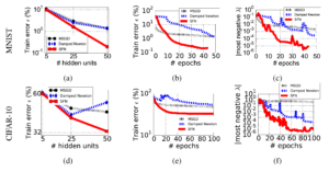
Based on the above figure, we can observe that:

In (a) and (d), as the number of hidden units increases, our model become much more high-dimensional. It’s obvious that both SGD and damped Newton method get stuck around a hidden unit number of 25. However, for their proposed SFN, it’s still able to step into a region of much lower error. This indirectly indicates that the number of saddle points increases exponentially as the dimensionality of model increases.
From (b) and (e) of learning curves plotted in terms of epochs, it confirms that SFN can evade away from saddle points and achieves a much lower training error. While for SGD and damped Newton method, both get trapped in regions where SFN does not.
Finally, from (c) and (f), the evolution of the absolute value of most negative eigenvalue is shown, which shows that it moves more toward the right as we achieve a lower error. So we are gradually having a more positive definite Hessian matrix. This indicates a local minimum instead of saddle points, for which we have successfully escaped.

The Effectiveness of Saddle-Free Newton Method

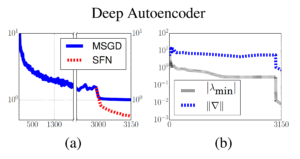
Furthermore, the authors tried to verify that their SFN method is also able to repel away from saddle points and achieves local minimum under deep neural networks. A seven-layer deep autoencoder is trained on the full-scale MNIST dataset, the approximate SFN jumps in after mini-batch SGD got stuck. The learning curve is shown in (a) of the figure below. We can also discover that after SFN is incorporated, the magnitude of the absolute value of the minimum eigenvalue and the norm of gradients have been reduced significantly.

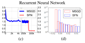
Recurrent Neural Network Optimization

In the end, the authors tried to test if SFN is able to help training the recurrent neural network (RNN) if the training difficulty is caused by saddle points. A small RNN with $120$ hidden units targeted for character-level language modeling is trained on the classical Penn Treebank dataset. Again SFN was used after SGD got trapped. A similar trend for learning curve is found as shown in (c) of the following figure. Furthermore, we can see in fig (d) that the Hessian matrix of the final solution found by SFN has much fewer negative eigenvalues as compared to ones found by mini-batch SGD.

Author: yufengma

Saddle-Points in Non-Convex Optimization