reidbix

AdaGrad is simply just an optimization method based off of the Proximal Point Algorithm (otherwise known as the Gradient Descent algorithm), specifically the Stochastic version of gradient descent. The intention behind the formulation of AdaGrad is because SGD (stochastic gradient descent) converges slowly in the cases when features of our model are significantly more important than others. This is because the original SGD algorithm treats all factors equally, regardless of how much each factor contributes towards the actual models outputs.

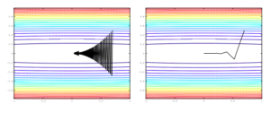
Seen below, we can recognize that the stochastic gradient descent algorithm takes a large amount of time in order to find the optimal solution because of the constant jumping back and forth on the expected gradient (seen Left). On the otherhand, if we were to average all of the iterates in SGD (not AdaGrad), we can find a much quicker optimization and decrease the amount of backtracking done.

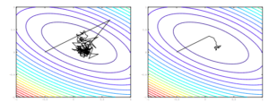
Now consider a case where we have an extremely wide problem domain, most likely due to a feature having an exaggerated effect on the domain. Seen below, we can see that the standard proximal gradient method (SGD) ends up jumping back and forth because it is a poorly conditioned problem. On the other hand, we can see the AdaGrad variant (which somewhat fixes the poor conditioning of the problem) will end up getting to the optimal in a significantly smaller number of steps.

The original SGD algorithm’s update method defines the update rule as:

$x^{(k+1)} = \text{argmin}_{x \in \chi} \{ \langle g^{(k)}, x \rangle + \frac{1}{2 \alpha_k} \lvert \lvert x - x^{(k)} \rvert \rvert_2^2 \}$

This version of the algorithm has a general convergence rate of $O(1/\sqrt{T})$

AdaGrad takes advantage of the matrix norm, in our case, $B$ will be a positive definite matrix such that:

$\lvert \lvert x \rvert \rvert^2_B := x^T Bx \geq 0$

This matrix $B$ has a list of diagonal terms that will modify the update rule of SGD such that:

$x^{(k+1)} = \text{argmin}_{x \in \chi} \{ \langle \nabla f(x^{(k)}), x \rangle + \frac{1}{2 \alpha_k} \lvert \lvert x - x^{(k)} \rvert \rvert_B^2 \}$

which is equivalent to an update rule of:

$x^{(k+1)} = x^{(k)} - \alpha B^{-1} \nabla f(x^{(k)})$

As can be seen when compared to the original update rule, we have introduced the diagonal matrix $B$ in order to converge more quickly because of the reliance on features that are more exaggerated than less important features. Now the question is how we can best approximate $B$, since it is unknown to the user.

AdaGrad now extends the SGD algorithm by defining within iteration $k$ :

$G^{(k)} = \text{diag} \lbrack \sum_{i=1}^{k} g^{(i)} (g^{(i)})^T \rbrack^{1/2}$

We can define $G^{(k)}$ as a diagonal matrix with entries:

$G^{(k)}_{jj} = \sqrt{\sum_{i=1}^{k} (g_j^{(i)})^2}$

Therefore modifying our previous modified update rule to be our final update rule for Adagrad:

$x^{(k+1)} = \text{argmin}_{x \in \chi} \{ \langle \nabla f(x^{(k)}), x \rangle + \frac{1}{2 \alpha_k} \lvert \lvert x - x^{(k)} \rvert \rvert_{G^{(k)}}^2 \}$

which is equivalent to an update rule of:

$x^{(k+1)} = x^{(k)} - \alpha G^{-1} \nabla f(x^{(k)})$

Proof of Convergence:

In order to go about proving that this new update rule will converge on the optimal solution just as SGD does, we must go about looking at the logic behind our choosing the diagonal matrix for our value of the matrix $B$.

To go about proving this we must have a couple of initial assumptions, definitions, and observations:

Assumption 1

$\vert \lvert x - x^{*} \rvert \rvert_{\infty} \leq R_{\infty}$ for all $x \in \chi$

Definition 1

(bound on the second moments of the $j$ th partial derivative of the function $F$ )

$\sigma_j^2 \geq E\lbrack (\nabla_j F(x;a_i))^2 \rbrack$ for all $x \in \chi$

Observation 1

$C \subset R^n$

$\pi_C^A (y) := \text{argmin}_{x \in C} \lvert \lvert x-y \rvert \rvert^2_A$

for any $x \in C$ then:

$\lvert \lvert \pi_C^A (y) - x \rvert \rvert^2_A \leq \lvert \lvert y - x \rvert \rvert^2_A$

Observation 2

$f$ is convex and differentiable such that:

$f(y) \geq f(x) + \langle f(x), y-x \rangle$

We utilize a theorem defined in the original paper which is also proved later on in the paper that suggests that given a step-size $\alpha = R_\infty$ and $\hat{x}_k = \frac{1}{k} \sum_{k=1}^{K} x_k$ such that:

Theorem 3

$E \lbrack f(\hat{x}_k) \rbrack - f(x^*) \leq \frac{2 R_\infty}{K} \sum_{j=1}^{n} E \lbrack ( \sum_{k=1}^{K} g_{k,j}^2 )^{1/2} \rbrack \leq 2 \frac{R_\infty \sum_{j=1}^{n} \sigma_j}{\sqrt{K}}$

The above equation is what we want to end up proving in order to show that the AdaGrad algorithm will converge on an optimal solution given enough steps $k$ .

Proof

Now that we’ve gone about and defined all of our required values, we can go about proving the convergence of the AdaGrad algorithm.

We first look at our update step of:

$x_{k+1} = \text{argmin}_{x \in \chi} \{ \langle g_k, x \rangle + \frac{1}{2\alpha} \lvert \lvert x - x_k \rvert \rvert^2_{G_k} \}$

which when projected into our problem space:

$\tilde{x}_{k+1} = x_k - \alpha G_K^{-1} g_k$

such that our new update step can be:

$x_{k+1} = \text{argmin}_{x \in \chi} \{ \lvert \lvert \tilde{x}_{k+1} - x \rvert \rvert^2_{G_k} \}$

This can be seen that the Potential Function is:

$\frac{1}{2} \lvert \lvert x_k - x^* \rvert \rvert^2_2$

And the AdaGrad Function would then be:

$\frac{1}{2} \lvert \lvert x_{k+1} - x^* \rvert \rvert^2_{G_k}$

Here, we’ll modify our AdaGrad function utilizing the previous definitions and the Potential function:

$\frac{1}{2} \lvert \lvert x_{k+1} - x^* \rvert \rvert^2_{G_k} \leq \frac{1}{2} \lvert \lvert x_k - \alpha G_k^{-1} g_k - x^* \rvert \rvert^2_{G_k}$

$= \frac{1}{2} \lvert \lvert \tilde{x}_{k+1} - x \rvert \rvert^2_{G_k}$

$= \frac{1}{2} \lvert \lvert x_k - x^* \rvert \rvert^2_{G_k} + \alpha \langle g_k, x^* - x_k \rangle + \frac{\alpha^2}{2} \lvert \lvert G_k^{-1} g_k \rvert \rvert^2_{G_k}$

$= \frac{1}{2} \lvert \lvert x_k - x^* \rvert \rvert^2_{G_k} + \alpha \langle g_k, x^* - x_k \rangle + \frac{\alpha^2}{2} \lvert \lvert g_k \rvert \rvert^2_{G_k^{-1}}$

We can see that the middle term of the final equation can be seen as:

$\langle g_k, x^* - x_k \rangle \leq f_k(x^*) - f_k(x_k)$

This rightmost term can be modfied to be:

$f_k(x^*) - f_k(x_k) \leq \frac{1}{2 \alpha} \lbrack \lvert \lvert x_k - x^* \rvert \rvert^2_{G_k} - \lvert \lvert x_k - \alpha G_k^{-1} g_k - x^* \rvert \rvert^2_{G_k} \rbrack + \frac{\alpha}{2} \lvert \lvert g_k \rvert \rvert^2_{G_k^{-1}}$

We can now modify this step with a summation of elements such that:

$\sum_{k=1}^{K} f_k(x^*) - f_k(x_k) \leq \frac{1}{2 \alpha} \sum_{k=1}^{K} \lbrack \lvert \lvert x_k - x^* \rvert \rvert^2_{G_k} - \lvert \lvert x_{k+1} - x^* \rvert \rvert^2_{G_k} \rbrack + \frac{\alpha}{2} \sum_{k=1}^{K} \lvert \lvert g_k \rvert \rvert^2_{G_k^{-1}}$

With this step, we can define $G_{k+1} \succeq G_k$ for all $k$ given that $G_k := \text{diag} (\sum_{i=1}^{K} g_i g_i^T)^{1/2}$ . With this definition we can now create a new Lemma:

$\sum_{k=1}^{K} \langle g_k, G_k^{-1} g_k \rangle \leq 2 \sum_{j=1}^{n} \sqrt{\sum_{k=1}^{K} g_{k,j}^2}$

Since we’ve expanded out our summation of elements above, we need to reduce our first term on the right side of the $\leq$ sign:

$\sum_{k=1}^{K} \lbrack \lvert \lvert x_k - x^* \rvert \rvert^2_{G_k} - \lvert \lvert x_{k+1} - x^* \rvert \rvert^2_{G_k} \rbrack = \lbrack \lvert \lvert x_1 - x^* \rvert \rvert^2_{G_1} - \lvert \lvert x_{k+1} - x^* \rvert \rvert^2_{G_k} \rbrack + \sum_{k=2}^{K} \lbrack \lvert \lvert x_k - x^* \rvert \rvert^2_{G_k} - \lvert \lvert x_{k} - x^* \rvert \rvert^2_{G_{k-1}} \rbrack$

The final term in the above equation is based off of the definitions of the norm and applying out when $G_k - G_{k-1}$ is needed to expand out our summation terms.

We use the basic definition of our space and the diagonal to form the defintion:

$\lvert \lvert y \rvert \rvert^2_{G_k} \leq \lvert \lvert \text{diag} (G_k) \rvert \rvert_1 \lvert \lvert y \rvert \rvert^2_\infty$

We use this definition in the final term of the previous equation that was expanded out in order to see that:

$\sum_{k=2}^{K} \lvert \lvert \text{diag}( G_k - G_{k-1} )\rvert \rvert_{1} \lvert \lvert x_{k} - x^* \rvert \rvert^2_\infty \leq \sum_{k=2}^{K} \lvert \lvert \text{diag}( G_k - G_{k-1} )\rvert \rvert_{1} R^2_\infty$

For better understanding we will define a new function:

$\text{tr} (X) = \lvert \lvert \text{diag} (X_k - X_{k-1}) \rvert \rvert_1$

Using the Assumption 1 we can now see that:

$\sum_{k=1}^{K} \lbrack \lvert \lvert x_k - x^* \rvert \rvert^2_{G_k} - \lvert \lvert x_{k+1} - x^* \rvert \rvert^2_{G_k} \leq R_\infty^2 \text{tr} (G_k) = R_\infty^2 \sum_{j=1}^{n} \sqrt{\sum_{k=1}^{K} g_{k,j}^2}$

Going back to one of our previous definitions, we can reduce this to:

$\sum_{k=1}^{K} f_k(x^*) - f_k(x_k) \leq \lbrack \frac{1}{2 \alpha} R_\infty^2 + \alpha \rbrack \sum_{j=1}^{n} \sqrt{\sum_{k=1}^{K} g_{k,j}^2}$

Given the fact that the potential function $E \lbrack f(x_k) | x_k \rbrack = f(x_k)$ we can now finally modify this to find our convergence proof that we were originally looking for:

$E \lbrack f(\hat{x}_k \rbrack - f(x^*) \leq \frac{1}{k} \lbrack \frac{1}{2 \alpha} R_\infty^2 + \alpha \rbrack E \lbrack \sum_{j=1}^{n} \sqrt{\sum_{k=1}^{K} g_{k,j}^2} \rbrack$

This proves that our given new update rule for AdaGrad will produce an optimal solution at (approximately) the same rate that SGD does.