nischelk

1. Introduction

This blog post covers analysis of Alternating Direction Method of Multipliers (ADMM); which solves Convex Optimization problems by breaking the problems into subproblems efficiently. Sections: ${1}$ to ${6}$ are written by Nischel Kandru and rest of them by Ahmadreza Azizi.

2. Dual Ascent

${\rightarrow}$ Consider the Convex Optimization problem which minimizes ${f(x)}$ such that ${Ax = b}$ .

Lagrangian for this problem is:
${L(x,y) = f(x) + y^T (Ax-b)}$

Dual problem of the original problem is:
${g(y)= max_{y} -f^{*}(-A^{T}y) -b^{T}y}$ , where ${f^*}$ is the convex conjugate of the objective function ${f}$ and ${y}$ is the dual variable or the lagrange multiplier.

${\rightarrow}$ If strong duality holds, then the optimal values of the primal and dual problems are the same.

${x^* = argmin_x \quad L(x,y^*)}$

where ${x^*}$ is the primal optimal point and ${y^*}$ is the dual optimal point; provided there is only one minimizer of ${L(x,y^*)}$ ( ${f}$ is strictly convex)

${\rightarrow}$ If ${f}$ is just convex (implies there isn’t a unique minimizer), instead dual-subgradient is performed rather than dual gradient;

${x^* \in argmin_x \quad L(x, y^*)}$

${\rightarrow}$ In the dual ascent method, to solve the dual problem, gradient ascent method would be used. Assuming ${g}$ is differentiable, we find:
${x^+ = argmin_x L(x,y)}$ and ${\nabla g(y) = Ax^+ - b}$

${\rightarrow}$ If ${g}$ is non-differentiable, we use sub-gradient method to solve the minimization problem:

${x^{k+1} = argmin_x L(x,y^k)}$ : x-minimization step
${y^{k+1} = y^k + \alpha^k (Ax^{k+1} - b)}$ : dual variable update,
where ${k}$ is the iteration step and ${\alpha^k}$ is the step sizes.

Repeat the above steps iteratively to solve the optimization problem. This is called dual ascent; because with appropriate step size ${\alpha^k}$ , we always get ${g(y^{k+1}) > g(y^k)}$ .

Let’s derive the above minimization steps:

Given ${f}$ , an objective function then the conjugate of the function: ${f^*(y) = max_{x \in R^n} \quad y^T x - f(x)}$ ; maximum over all points ${x}$ evaluated at point ${y}$ .

If ${f}$ is closed and convex, then ${f^{**} = f}$ ; conjugate of conjugate is the function itself. Also, ${x \in \partial f^* (y)}$ if and only if ${y \in \partial f(x)}$ if and only if ${x \in argmin_x f(x) - y^Tx}$ ; if ${x}$ is the subgradient of the conjugate at ${y}$ , if and only if ${y}$ is the subgradient of the original function at ${x}$ .

${x \in \partial f^*(y)}$ if and only if ${x \in argmin_x f(x) -y^Tx}$ , sub-gradient for maximum is the one that achieves the maximum. We also know that achieving maximum is same as achieving minimum; so
${x \in argmin_x -(y^Tx - f(x))}$
${\implies x \in argmin_x (f(x) - y^Tx)}$

Dual problem:
${g(y) = max_y -f^*(-A^Ty) - b^Ty}$ — (1)
Suppose ${G(y) = f^*(-A^Ty)}$
Subgradients of (1) are: ${\partial G(y) - b}$ where;
${\partial G(y) = A \partial f^* (-A^Ty)}$
${x \in \partial F^* (-A^Ty)}$ if and only if ${x \in argmin_x f(x) + y^TAx}$

${x^{k+1} \in argmin_x f(x) + {y^k}^TAx}$
${\implies x^{k+1} \in L(x,y^k)}$
${y^{k+1} = y^k + \alpha^k (Ax^{k+1} -b)}$

Disadvantages of Dual Ascent

Slow Convergence
Even though we may achieve convergence in dual objective value, convergence of ${y^k}$ , ${x^k}$ to solutions require strong assumptions

Advantages of Dual Ascent
Decomposability; which leads to Dual Decomposition

3. Dual Decomposition

If ${f}$ is separable, then dual ascent can be decentralized.

${f(x) = \sum_{i=1}^{N} f_i (x_i)}$

The Lagrangian for this problem would be:

$\displaystyle L(x,y) = \sum_{i=1}^{N} L_i (x_i, y) = \sum_{i=1}^{N} (f_i (x_i) + y^TA_ix_i - (1/N)y^Tb)$

$\displaystyle {x_i}^{k+1} := argmin_{x_i} L_i(x_i, y^k)$

we can compute the x-minimization steps in parallel, thanks to the decomposability.

$\displaystyle y^{k+1} := y^k +\alpha^{k} (Ax^{k+1} -b)$

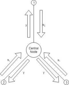
This essentially involves couple of steps:

Broadcast: Send ${y}$ to each of the other nodes, each optimizes in parallel to find ${x_i}$
Gather: Collect ${A_ix_i}$ from each node, update the global dual variable ${y}$

4. Augmented Lagrangian and Method of Multipliers

To yield convergence without assumptions like strict convexity, we add a new term; so that the function becomes more convex.

$\displaystyle L_{\rho} (x,y) = f(x) + y^T(Ax-b) + \frac{\rho}{2}{||Ax-b||_2}^2$

where ${\rho > 0}$ is the penalty parameter

We can clearly see that the addition of the new term doesn’t change the problem as such, because the constraint is ${Ax=b}$ . The new term provides:

Numerical Stability
Smooths out the primal criterion function
Introduces curvature into the objective function

Augmented Lagrangian can be viewed as the Lagrangian with problem-

$\displaystyle min \quad f(x) + \frac{\rho}{2}{||Ax-b||_2}^2$

subject to ${Ax = b}$

${\rightarrow}$ With the penalty term ${\rho}$ , dual function ${g_\rho}$ can be shown to be differentiable under rather mild conditions on the original problem.

${\rightarrow}$ Applying dual ascent yields:

${x^{k+1} := argmin_x L_\rho (x,y^k)}$
${y^{k+1} := y^k + \rho (Ax^{k+1} -b)}$

${\rightarrow}$ Optimality conditions for original problem are primal and dual feasibility, i.e,

$\displaystyle Ax^* - b = 0, \nabla f(x^*) + A^Ty^* = 0$

Let’s see the motivation behind having ${\rho}$ as the stepsize instead of ${\alpha^k}$ .

${\nabla L_\rho {(x, y^k)}_{x=x^{k+1}} = 0}$ , since ${x^{k+1}}$ minimizes
${\nabla f(x^{k+1}) + A^Ty^k + \rho A^T (Ax^{k+1} - b) = 0}$
${\nabla f(x^{k+1}) + A^T(y^k + \rho(Ax^{k+1} - b)) = 0}$
${\nabla f(x^{k+1}) + A^T(y^{k+1}) = 0}$
${(x^{k+1}, y^{k+1})}$ is dual feasible

${\rightarrow}$ This is the stationary condition for original problem, so to preserve this use ${\rho}$ as stepsize.
${\rightarrow}$ We get much better convergence in Augmented Lagrangian, but lose out on the decomposability; the solution to this is ADMM which gets the best out of both the worlds.

5. Alternating Direction Method of Multipliers

ADMM combines Decomposability of Dual Ascent and the convergence of Method of Multipliers.

$\displaystyle min \quad f(x) + g(z)$

where ${f}$ and ${g}$ are convex, subject to ${Ax+Bz=c}$

The Lagrangian for this problem is:
${L_\rho (x,z,y) = f(x) + g(z) + y^T(Ax+Bz-c) + \frac{\rho}{2}{||Ax+Bz-c||_2}^2}$

${x^{k+1} := argmin_x L_\rho (x, z^k, y^k)}$ — X- minimization step
${z^{k+1} := argmin_z L_\rho (x^{k+1}, z, y^k)}$ — Z- minimization step
${y^{k+1} := y^k + \rho (Ax^{k+1} + Bz^{k+1} -c)}$ — dual variable update step

${\rightarrow}$ ${x}$ and ${z}$ are updated in an alternating fashion.
${\rightarrow}$ We can clearly see that the Z- minimization step depends on the updated value ${x^{k+1}}$ ; so these steps cant be parallelized completely.

The method of multipliers for this problem would have the form:

$\displaystyle (x^{k+1}, z^{k+1}) := argmin_{x,z} L_\rho (x,z,y^k)$

$\displaystyle y^{k+1} := y^k + \rho (Ax^{k+1} +Bz^{k+1} -c)$

we can clearly see that, here we try to minimize ${x}$ and ${z}$ together and lose out on the decomposability.

${\rightarrow}$ We force decomposability in ADMM, we dont have complete power of decomposability as ${z^{k+1}}$ depends on ${x^{k+1}}$ but we can compute all the ${x_i}$ s and ${z_i}$ s parallely.

${\rightarrow}$ We can see that ADMM doesnt converge as much as the Method of Multipliers and doesnt decompose as much as Dual Decomposition. But, it takes the best of both worlds.

${\rightarrow}$ ADMM in general requires lot of iterations for highly accurate solutions, but obtains relatively accurate solution in few iterations.

Scaled Form
We can have a scaled dual variable as: ${u= \frac{1}{\rho}y}$ and this makes the computations efficient.

$\displaystyle x^{k+1} := argmin_x (f(x) + \frac{\rho}{2}{||Ax+Bz^k-c+u^k||_2}^2)$

$\displaystyle z^{k+1} := argmin_z (g(z) + \frac{\rho}{2}{||Ax^{k+1}+Bz-c+u^k||_2}^2)$

$\displaystyle u^{k+1} := u^k + Ax^{k+1} +Bz^{k+1} -c$

6. References

http://stanford.edu/~boyd/admm.html
http://www.stat.cmu.edu/~ryantibs/convexopt-F13/lectures/23-dual-meth.pdf