During our introductory lecture on submodular functions, based on Francis Bach’s paper, we discussed the importance of combinatorial optimization for machine learning applications, reviewed set notation, and defined the key concepts from chapters 2-3 of Bach’s paper.
Importance of Combinatorial Optimization for Machine Learning
Feature selection, factoring distributions, ranking, clustering, and graph cuts were given as examples of machine learning problems that are combinatorial by nature and require either maximization or minimization. When discussing the importance of submodular functions and combinatorial optimization, we referred to the feature selection example from this slide deck produced by professors Andreas Krause and Carlos Guestrin.
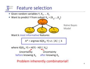
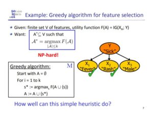
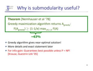
In the feature selection example, we desire to choose the k best features that will add the most certainty in predicting the dependent variable (in this example, Y = “Sick”). As Krause and Guestrin point out, this problem is inherently combinatorial and therefore requires combinatorial optimization techniques. The goal of choosing an optimal feature set, |A*| ≤ k, is outlined in the first two slides. The problem is NP-hard because there are (2^p) – 1 constraints so we use a greedy algorithm to solve it. This essentially means that we take the best individual element that minimizes the marginal uncertainty of adding it to the current optimal set, A*. We repeat this process for up to k iterations until our optimal set is finalized. Although this certainly isn’t going to give us the true optimal set every time because some combinations of features may be more optimal when paired together, Krause and Guestrin inform us that it does give us a guarantee of at least 1 – 1/e (~63%) sub-optimal performance.
Background
Before covering the Bach paper material, we reviewed set function notations for those people who hadn’t taken a discrete math or combinatorics class. The slide below outlines the notations covered during our class lecture.
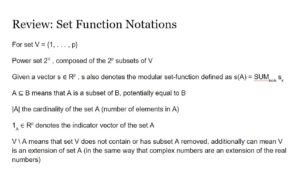
The three notations at the bottom of the slide seemed to be the ones that students were least familiar with. Cardinality (absolute value signs around a set) is simply the number of elements contained within a given set. The indicator vector, 1_A, for the set A is simply a vector with a 1 in a particular dimension if the element corresponding to that vector dimension is contained in the set A and is a 0 if it isn’t. Lastly, the notation V \ A is simply set V with subset A removed.
Submodular Functions and the Lovász Extension
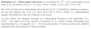
When we introduced submodular function notation, we used both Definition 2.1 and Proposition 2.2 from the book. When first learning about submodularity, we found that the proposition 2.2, which introduces the property of diminishing returns, was more intuitive and made understanding definition 2.1 easier.
![]()
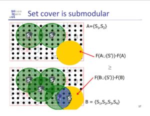
To further ring home the concept of submodular functions and the property of diminishing returns, we reviewed the set cover example from the Krause and Guestrin slides below. The goal of this visual aid was to demonstrate how adding a new element to a set A, a subset of set B, can only cover the same or more surface area than adding the same new element to set B.
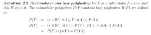
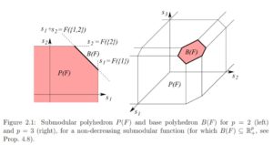
During the next part of the lecture, we reviewed associate polyhedra which was by far the most confusing material to cover for the class. The differences between submodular and base polyhedra expressed in Bach’s paper is clear to understand. The base polyhedra, B(F), can be thought of as the hollow outer shell of the set function formed by the intersecting constraint hyperplanes and the submodular polyhedra, P(F), can be thought of as the base polyhdra and the discrete, encapsulated, non-empty interior space encompassed by the base polyhedra. What we found confusing was whether Figure 2.1 below was representing just the domain of the set function, F, or if it was also representing the function values. We agreed that we thought the figure was only representing the domain, because it would need an additional dimension to represent the set function values for the elements s1, s2, and s3.
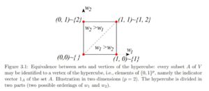
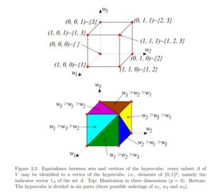
Finally, we had the opportunity to introduce the Lovász extension (also referred to as the Choquet integral) which allows us to extend the vertices of a {0,1}^p hypercube to a continuous [0, 1]^p hypercube (think of taking the convex hull of the vertices). By dividing the continuous hypercube into p! simplices, we can create areas with ordered variable values like in the figures from Bach’s paper below.
One of the last things we were able to cover in class was the properties of the Lovász extension. The Lovász extension is important mainly because it allows us to create a continuous extension of discrete problems. Additionally, it has a unique connection with submodularity and convexity. A set function is submodular if and only if its Lovász extension is convex. We ended the class by proving this theorem.
Theorem: A set-function, F, is submodular if and only if its Lovász extension, f, is convex.

Proof: Let's assume f is convex. Let A, B ⊆ V. The vector,
![]()
has components equal to 0 where [ V \ (A ∪ B) ]
                        2 where [ A ∩ B ]
                    and 1 where [ A Δ B = (A \ B) ∪ (B \ A) ].

Using the property,
![]()
we get
![]()
![]()
![]()
![]()
Since f is convex, then
![]()
=![]()
Therefore, F(A) + F(B) = F(A ∪ B) + F(A ∩ B). This satisfies the definition of convexity, therefore if F is submodular, then it is sufficient that for all ω ϵ ℝ^p, f(ω) is a maximum of linear functions, thus it is convex on ℝ^p.