Introduction
The convex-concave saddle point problem has the following format:
![]()
For many machine learning applications, their objective functions can be written in the convex-concave format. The example applications include reinforcement learning, empirical risk minimization and robust optimization etc.
We can use the following primal-dual gradient method to optimize the .
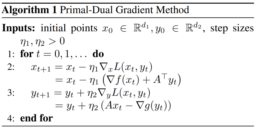
In this paper, the authors develop a new method to prove that the primal-dual gradient method has linear convergence rate, when the and
are smooth,
is convex,
is strongly convex and the coupling matrix
has full column rank(Section 3). They also extend the primal-dual method to the stochastic situation and propose the primal-dual stochastic variance reduced gradient(SVRG) method. They use the new method to prove that the primal-dual SVRG method also has linear converge rate(Section 4).
Preliminaries
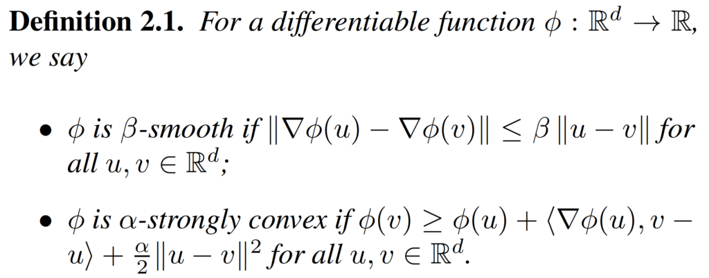
Before we prove the convergence of the primal-dual method, we need some preliminaries. First, we need the definitions of smoothness and strong convexity.
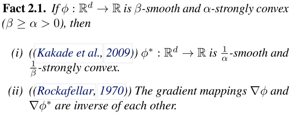
We also need the definition and some properties of the conjugate function.

Based on the definition of conjugate function, we can get the corresponding primal problem of the .
![]()
Finally, we need the of gradient descent on the strongly convex function.

Linear Convergence of the Primal-Dual Gradient Method
With these preliminaries, we can start to prove the convergence of primal-dual gradient method. The Theorem 3.1 establishes the linear convergence guarantee for it.
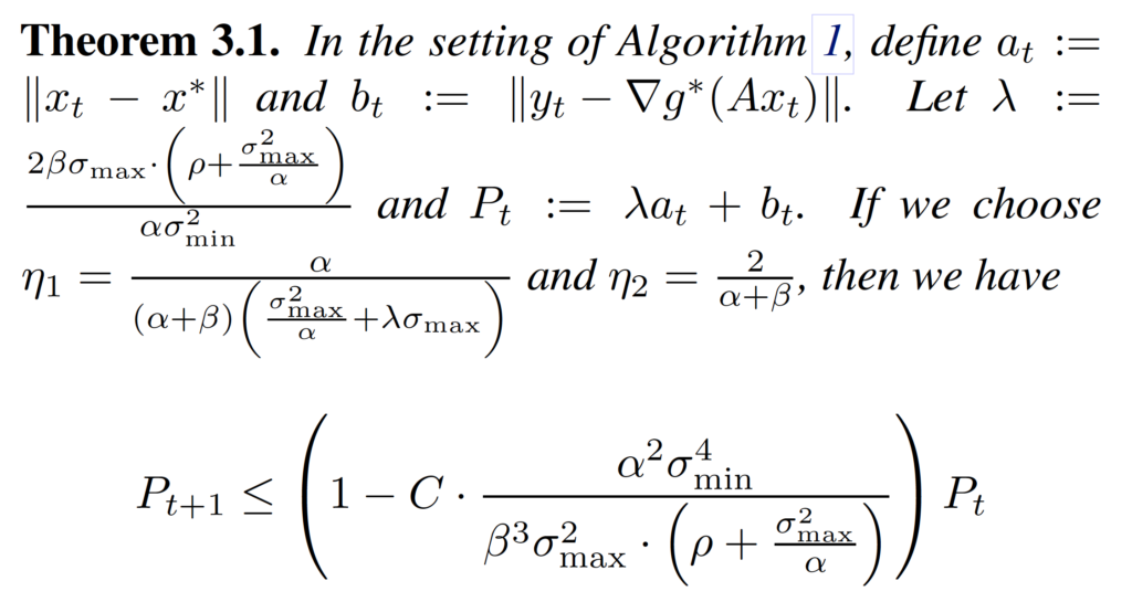
This theorem says that if we construct a Lyapunov function , we can prove that the function satisfies the condition that
, which implies the linear convergence rate.
We can divide the proof of this theorem to three steps. First, we bound the decrease of . That is, we want to prove that
. Second, we bound the decrease of
. Finally, we prove the inequality.
Proposition 3.1 and Proposition 3.2 give the bound of decrease of .


The proof technique of the first step is to first find the relationship between and
, and the relationship between
and
. And then use the triangle inequality to find the relationship among
,
and
. The authors call the
ghost variable in this paper, which is actually the $x$ obtained by updating the
with the true gradient, i.e.,
.
Proposition 3.3 and Proposition 3.4 give the bound of decrease of . We can use the convex function’s property to prove them.
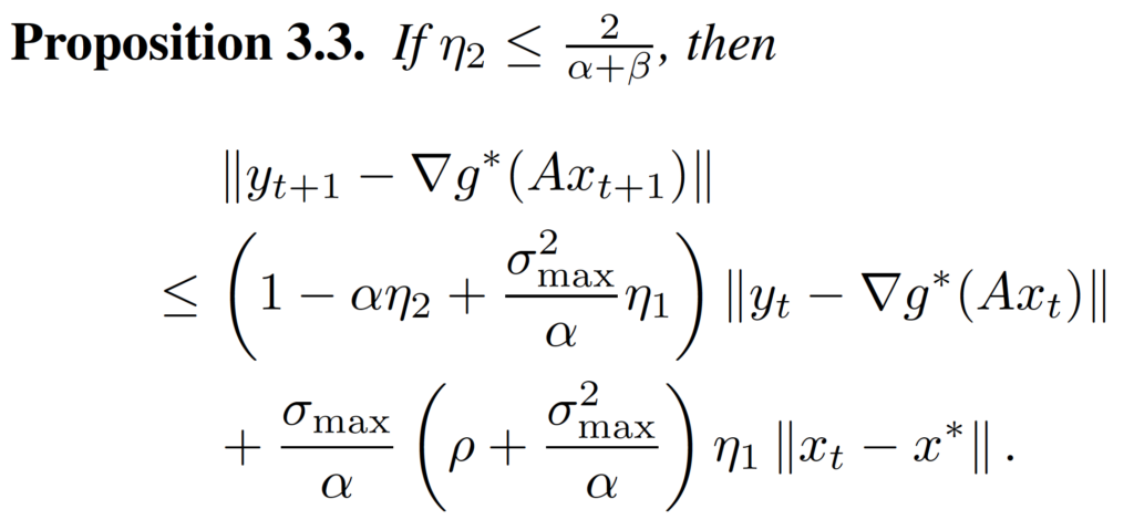

After we have these propositions, we can put them together, and with some routine calculations, we can prove the inequality in Theorem 3.1.
Extension to the Primal-Dual Stochastic Variance Reduced Gradient Method
In this section, the authors propose the primal-dual SVRG, and prove its convergence using the same proof method in the third section. The primal-dual SVRG is in Algorithm 2.
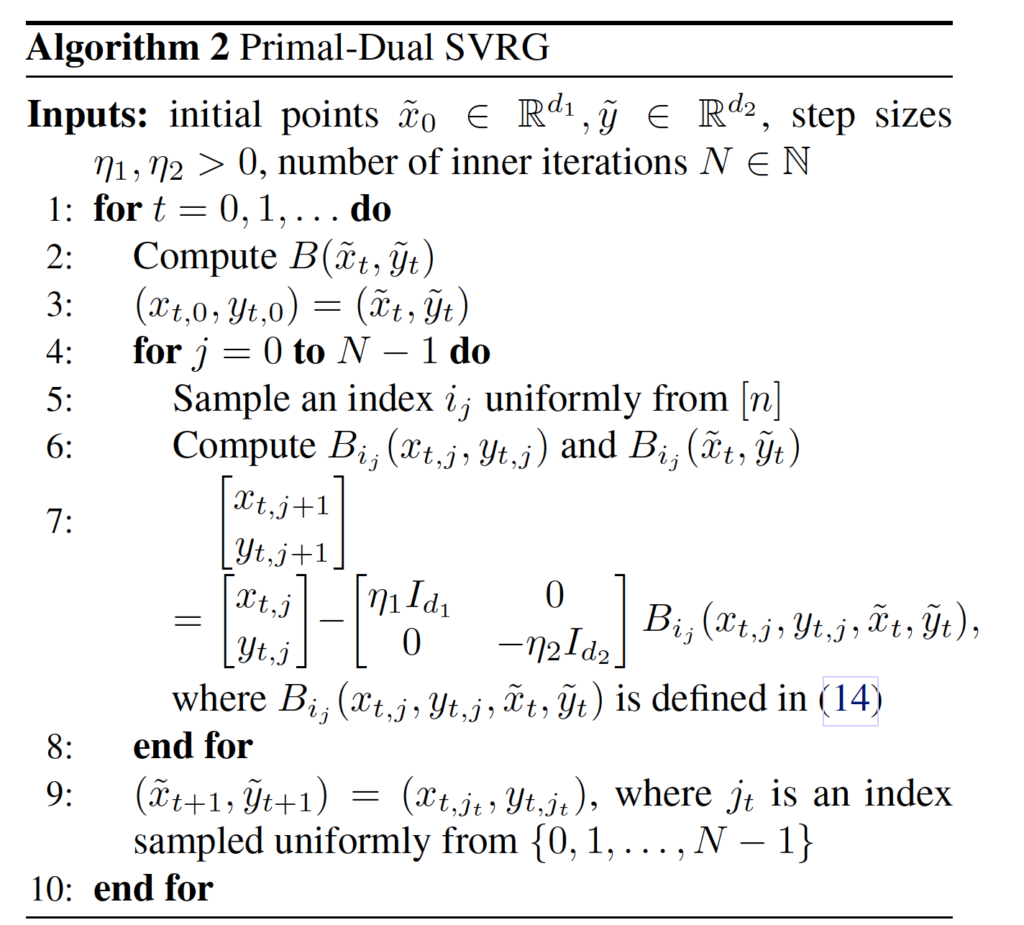
The framework of primal-dual SVRG is the same as the vanilla SVRG. The main difference is only that the primal-dual SVRG updates the parameters and
together. In Theorem 4.1, they prove that the primal-dual SVRG also has the linear convergence rate.
Preliminary Empirical Evaluation
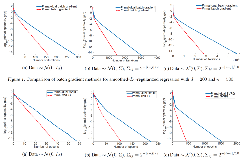
They do experiments on synthetic dataset to prove the convergence of primal-dual gradient method. The results are as below.
