1.Background
Zhang et al. (2016) observed a very “surprising” result. They trained a deep network and they took the same input images, but randomized the labels, and found that their networks were not able to predict the test set, they still memorized the training labels. This result raise a question: why they can work well even though the models assign the label randomly?
Some useful results:
- hold the learning rate fixed and increase the batch size, the test accuracy usually falls.
- a linear scaling rule between batch size and learning rate
- a square root rule on theoretical grounds
2. Empirical principle
- “broad minima”>”sharp minima”:curvature of “broad minima” is small
- stochastic gradient descent (SGD) finds wider minima as the batch size is reduced.
- the curvature of a minimum can be arbitrarily increased by changing the model parameterization
In this paper, they consider the following two questions from a Bayesian perspective
a) how can we predict if a minimum will generalize to the test set?
b) why does stochastic gradient descent find minima that generalize well?
3.Bayesian Model Comparison
We consider a classification model with a single parameter ω

The first equation is the formula of the posterior distribution; the second equation is the likelihood and we choose Gaussian as prior.
Therefore, we can write the posterior distribution as below:

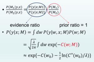
Given a new input $x_t$ to predict an unknown label $y_t$, we need to compute the integrals, however, these integrals are dominated by the region near$w_0$, so the integral can be approximately computed as above.
Probability ratio:

The second factor on the right is the prior ratio, which describes which model is most plausible. To avoid unnecessary subjectivity, we usually set this to 1. Meanwhile the first factor on the right is the evidence ratio, which controls how much the training data changes our prior beliefs. To calculate evidence P(y|x;M),we need the integral based on w. Since this integral is dominated by the region near the minimum w_0, we can estimate the evidence by Taylor expanding ![]() and “Laplace” approximation. Finally, we get the evidence for a model with a single parameter.
and “Laplace” approximation. Finally, we get the evidence for a model with a single parameter.
Then we can generalize this to model with many parameters as blow:

“Occam factor” enforces Occam’s razor: when two models describe the data equally well, the simpler model is usually better.
Next, we need to compare model M with Null model where all the label are randomly assigned with equal probability. We can get the evidence ratio:

E(w_0) is the log evidence ratio in favor of the null model.
From these formulas, we can get:
- broad minima generalize better than sharp minima, but not depend on the parameters
- need to rescale \lambda_i,\lambda to keep the model same
- hard to evaluate for deep networks for there are millions of parameters
4.Bayes Theorem and Generalization
- Consider a simple: logistic regression with label 0/1.
Task a: the labels of both the training and test sets are randomized.
Task b: the labels are informative, matching the true label
- replicating the observations of Zhang et al. (2016) in deep networks
Experiment results:
Figure 1 shows us that the model perfectly memorizes the random model.

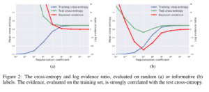
Figure 2(a) shows us that the model can never be expected to generalize well, 2(b) the model is much better than the NULL model according to the Bayesian evidence and cross-entropy.
Reference:
- A BAYESIAN PERSPECTIVE ON GENERALIZATION AND STOCHASTIC GRADIENT DESCENT
- related material